Kaldor and Goodwin’s Models of Business Cycles

INTRODUCTION

• J.R. Hicks explained business cycles through the interaction of multiplier and accelerator, constrained by a ceiling (full-employment level of output) and a floor (minimum level of economic activity), and integrated cyclical fluctuations with long-term economic growth.

• Hicks’s model is a non-linear dynamic framework where output fluctuates around a rising growth trend due to multiplier–accelerator interaction subject to upper and lower bounds.

• Kaldor developed another significant Keynesian non-linear model of business cycles, modifying the rigid accelerator assumption and providing a more flexible dynamic structure.

• R.M. Goodwin also proposed a non-linear dynamic growth-cycle model, explaining cyclical fluctuations around a steady growth path similar to Hicks but with different structural assumptions.

• Milton Friedman presented a monetarist theory of trade cycles, analyzing business fluctuations through changes in money supply and monetary disturbances rather than multiplier–accelerator interaction.

• Thus, major modern theories of business cycles include Hicks’s growth-cycle model, Kaldor’s non-linear Keynesian model, Goodwin’s dynamic growth-cycle model, and Friedman’s monetarist explanation based on monetary factors.

KALDOR’S MODEL OF BUSINESS CYCLE

• In Kaldor’s model of trade cycles, economic activity (aggregate output and employment) is determined by the interaction of specially shaped saving and investment functions.

• The equilibrium level of income is obtained where saving equals investment:
  $$S(Y) = I(Y)$$

• Both saving and investment functions are non-linear and possess peculiar shapes, unlike the simple linear forms used in basic Keynesian models.

• The intersection of these saving and investment curves yields three equilibrium points: two stable equilibria and one unstable equilibrium.

• The stable equilibria represent positions toward which the economy tends to move after a disturbance, while the unstable equilibrium represents a point from which the economy diverges when disturbed.

• Thus, cyclical movements in income and employment arise from the non-linear interaction of saving and investment functions around these multiple equilibrium points.

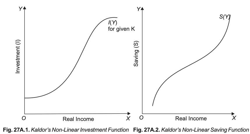
Kaldor’s Investment Function

• In Kaldor’s investment function, investment depends on the level of income (economic activity) and the stock of capital:
  $$I = f(Y, K),$$
  where \(\frac{\partial I}{\partial Y} > 0\) and \(\frac{\partial I}{\partial Y}\) represents the marginal propensity to invest.

• Unlike the rigid accelerator principle \(\big(I = v(Y_t – Y_{t-1})\big)\), Kaldor relates investment to the level of income rather than the rate of change of income. Thus, investment depends on aggregate output or employment itself, not merely on its growth.

• Kaldor incorporates the effect of capital accumulation on productive capacity and entrepreneurial decisions; higher capital stock reduces profitable investment opportunities, making the investment function non-linear.

• The non-linear investment curve shows a normal or moderate marginal propensity to invest in the middle range of income, but marginal investment propensity is low at both very low and very high levels of economic activity.

• At low income levels, weak profit expectations reduce investment responsiveness; at high income levels, diminishing economies of scale and rising financial costs lower marginal propensity to invest.

• Kaldor also assumes an inverse relationship between investment and capital stock:
  $$\frac{\partial I}{\partial K} < 0.$$
  As capital stock accumulates, productive capacity expands and investment opportunities shrink, causing the investment function to shift downward.

• Therefore, continuous capital accumulation reduces investment at each level of income, reinforcing the non-linear character of the investment function, which plays a central role in generating trade cycles in Kaldor’s model.