Budget Constraint | Micro Economics | Hal Varian

The Budget Constraint

• Consumer theory assumes that consumers choose the best bundle of goods they can afford. To explain this theory, two questions must be answered: what is meant by “best” and what is meant by “can afford.” This chapter focuses on what consumers can afford, while the next chapter explains how consumers determine what is best, providing the foundation for a detailed analysis of consumer behavior.

• The concept of what a consumer can afford is explained through the budget constraint. Although consumers can choose from many goods in reality, analysis is simplified by considering only two goods, making the consumer’s choice behavior easy to represent graphically.

• A consumer’s consumption bundle is represented as (x₁, x₂), where x₁ denotes the quantity of good 1 consumed and x₂ denotes the quantity of good 2 consumed. The bundle may also be written simply as X, where X is an abbreviation for the ordered pair (x₁, x₂).

• The analysis assumes that the prices of the two goods, (p₁, p₂), and the consumer’s income (m) are known. The consumer’s budget constraint is expressed as p₁x₁ + p₂x₂ ≤ m, where p₁x₁ is the amount spent on good 1 and p₂x₂ is the amount spent on good 2.

• The budget constraint requires that the total expenditure on both goods must be no greater than the consumer’s available income (m). Any consumption bundle satisfying this condition is affordable.

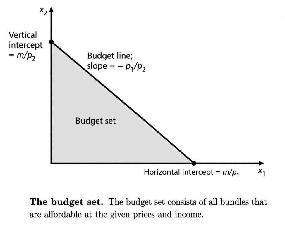
• The collection of all affordable consumption bundles, given the prices (p₁, p₂) and income m, is called the budget set of the consumer.

Two Goods are Often Enough

• The assumption of two goods is more general than it initially appears because one good can be interpreted as representing all other goods the consumer may wish to consume, allowing many real-world consumption problems to be analyzed with a two-good model.

• For example, when analyzing a consumer’s demand for milk, x₁ can represent the quantity of milk consumed (e.g., quarts per month), while x₂ represents everything else the consumer wishes to consume.

• Under this interpretation, good 2 is treated as the money available to spend on all other goods, making its price equal to 1, since one dollar costs one dollar. The budget constraint therefore becomes p₁x₁ + x₂ ≤ m.

• The expression p₁x₁ + x₂ ≤ m means that the amount spent on good 1 (p₁x₁) plus the amount spent on all other goods (x₂) cannot exceed the consumer’s total income (m).

• Good 2 is called a composite good, representing all goods other than good 1, and is always measured in dollars spent on those other goods rather than in physical units.

• From the algebraic perspective, the budget constraint p₁x₁ + x₂ ≤ m is simply a special case of the general budget constraint p₁x₁ + p₂x₂ ≤ m, where p₂ = 1. Since only the value of p₂ changes, all general results and analyses of the budget constraint remain valid under the composite-good interpretation.

Properties of the Budget Set

• The budget line is the set of all consumption bundles that exactly exhaust the consumer’s income, and is represented by the equation:
  [
  p_1x_1 + p_2x_2 = m.
  ]
  Every bundle on the budget line costs exactly (m), while all bundles below the budget line cost less than (m) and therefore belong to the budget set.

• Rearranging the budget line equation into slope-intercept form gives:
  [
  x_2=\frac{m}{p_2}-\frac{p_1}{p_2}x_1.
  ]
  This equation represents a straight line with:

  • Vertical intercept:
    [
    \frac{m}{p_2},
    ]
    showing the maximum quantity of good 2 that can be purchased if all income is spent on good 2.

  • Slope:
    [
    -\frac{p_1}{p_2},
    ]
    showing how much of good 2 must be given up when consuming additional units of good 1 while remaining within the budget.

  • The equation also indicates the quantity of good 2 the consumer can consume for any chosen quantity of good 1 while exactly satisfying the budget constraint.

• The budget line can be drawn easily using its intercepts:

  • If all income is spent on good 2, the maximum purchasable quantity is:
    [
    \frac{m}{p_2},
    ]
    which is the vertical intercept.

  • If all income is spent on good 1, the maximum purchasable quantity is:
    [
    \frac{m}{p_1},
    ]
    which is the horizontal intercept.

  • Plotting these two intercepts on the graph and joining them with a straight line gives the complete budget line.

• The slope of the budget line has an important economic interpretation because it measures the rate at which the market allows substitution between the two goods while keeping total expenditure unchanged. If the consumer increases consumption of good 1 by:
  [
  \Delta x_1,
  ]
  and changes consumption of good 2 by:
  [
  \Delta x_2,
  ]
  while continuing to satisfy the budget constraint, then:
  [
  p_1x_1+p_2x_2=m,
  ]
  before the change, and
  [
  p_1(x_1+\Delta x_1)+p_2(x_2+\Delta x_2)=m,
  ]
  after the change.

• Subtracting the original budget equation from the new one gives:
  [
  p_1\Delta x_1+p_2\Delta x_2=0.
  ]
  This means that the total value of the change in consumption is zero, so any increase in spending on one good must be exactly offset by a decrease in spending on the other good to remain on the budget line.

• Solving for the rate of substitution between the two goods gives:
  [
  \frac{\Delta x_2}{\Delta x_1}=-\frac{p_1}{p_2}.
  ]
  This is exactly the slope of the budget line, indicating the quantity of good 2 that must be sacrificed for each additional unit of good 1 while keeping total expenditure constant.

• The negative sign in the slope,
  [
  -\frac{p_1}{p_2},
  ]
  reflects that (\Delta x_1) and (\Delta x_2) must always have opposite signs to satisfy the budget constraint. Consuming more of good 1 requires consuming less of good 2, and consuming more of good 2 requires consuming less of good 1.

• Economists interpret the slope of the budget line as the opportunity cost of consuming good 1. Every additional unit of good 1 requires giving up some quantity of good 2, and this sacrificed consumption of good 2 represents the true economic cost of obtaining more of good 1. The magnitude of this opportunity cost is measured by:
  [
  \left|\frac{p_1}{p_2}\right|,
  ]
  while the slope itself is:
  [
  -\frac{p_1}{p_2}.
  ]