Consumption Function | UGC NET Economics – Notes

Introduction

The Consumption Function occupies a central place in Keynesian economic theory and forms one of the fundamental building blocks of the theory of income and employment determination. It was introduced by John Maynard Keynes in his book The General Theory of Employment, Interest and Money (1936) as part of his broader critique of Classical economics. The consumption function describes the functional relationship between the level of income and the level of consumption expenditure in an economy. Since consumption expenditure constitutes the largest component of aggregate demand, understanding the behaviour of consumption in relation to income is essential for understanding how the equilibrium level of output and employment is determined.

Meaning and Definition

The consumption function, also referred to as the propensity to consume, expresses the relationship between the aggregate consumption expenditure (C) of a community and the aggregate level of income (Y). Symbolically, it is expressed as:

C = f(Y)

This equation states that consumption is a function of income, that is, the amount spent on consumption depends upon the level of income earned. As income changes, consumption expenditure also changes, though not necessarily in the same proportion.

Equilibrium and Aggregate Demand

• We already know that the total demand for goods and services is known as aggregate demand. The factors which together make aggregate demand (AD) are consumption (C), investment (I), government expenditure (G), and net exports (NX).

  $$AD = C + I + G + NX$$

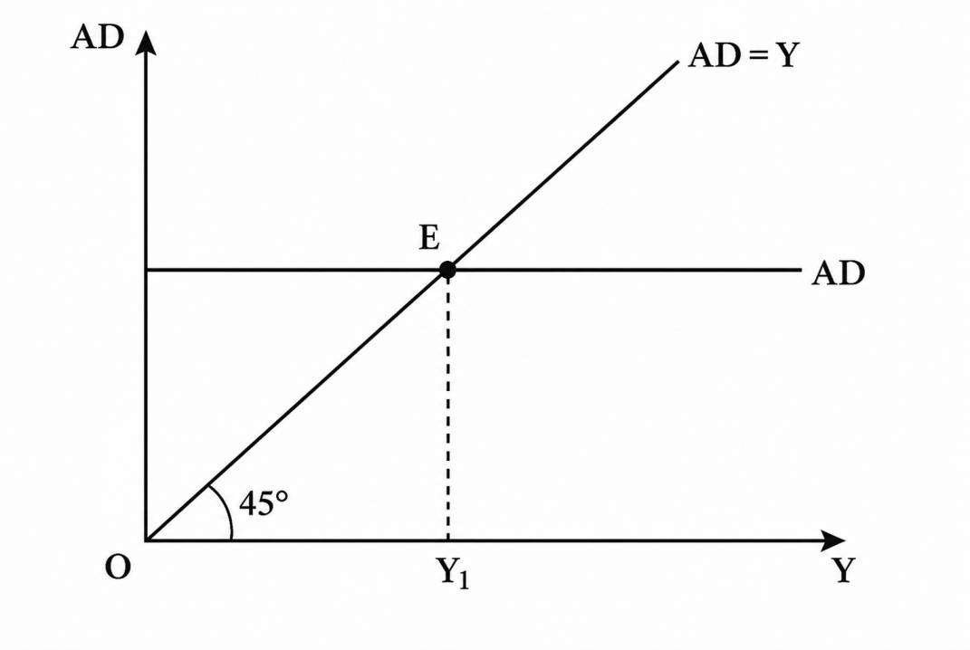
• In case we assume the aggregate demand for goods and services to be constant, we get a horizontal AD curve. It means that AD is independent of income and output levels. In Fig. 1, output level (representing aggregate supply) is presented on the x-axis while aggregate demand is shown on the y-axis. A 45° line shows equality between the variables shown on x-axis and y-axis, i.e., at any point on this 45° line,

  $$AD = Y$$

  In other words, this line represents the locus of equilibrium points where aggregate demand is equal to the output level. In case the AD curve is horizontal, we can say that the equilibrium exists at point E where

  $$AD = Y$$

  No forces are causing any change at point E. Equilibrium level of output is \(Y_1\).

• In case firms produce to the left of \(Y_1\), aggregate supply is less than aggregate demand, and there is run down of exiting inventories. On the other hand, if firms produce to the right of \(Y_1\), there is excess supply (aggregate supply is more than aggregate demand) and inventories will increase. In both the cases, there will be a movement towards (Y_1). At E, the firms are selling exactly what people demand. In case of a deviation from \(Y_1\), we have positive or negative unplanned inventory investment.

• Unplanned inventory investment is given by:

  $$UI = Y – AD$$

  where UI is unplanned inventory.

• When (Y > AD), we find that UI is positive, i.e., there is an addition to the stock of inventory. When (Y < AD), we find that UI is negative, i.e., the existing inventory is to be used in order to meet the aggregate demand. It is also called unplanned inventory disinvestment. This leads us to the equilibrium condition:

  $$Y = AD$$

• At equilibrium, there is no unplanned inventory investment. Aggregate demand is also indicated by planned spending. Hence, we can say that at equilibrium, planned spending equals income.