Inflation and Hyperinflation: Causes, Effects and Cure

Meaning of Inflation

• Inflation refers to a persistent rise in the general price level, not a one-time increase, while deflation means persistently falling prices.

• When inflation occurs, the value of money falls, as more money is required to purchase the same quantity of goods and services, increasing the cost of living.

• To maintain their standard of living during rising prices, people’s incomes must increase; government employees receive higher dearness allowance, and organised private sector wages and salaries are raised, though usually after a time lag.

• However, people with fixed incomes and many self-employed individuals cannot easily increase their earnings and therefore suffer losses in real income, with the poor being the worst affected, especially due to rising prices of foodgrains and essential commodities.

• India experienced particularly high rates of inflation during the 1970s and 1980s compared to earlier periods, making it a serious and persistent economic problem.

• In recent years such as 2010–11, 2011–12, and 2012–13, inflation in India, measured by the Consumer Price Index (CPI), reached double-digit levels, and even WPI inflation remained high before January 2013, prompting the Reserve Bank of India to adopt a tight monetary policy.

Causes of Inflation

• Inflation originates from different causes and is broadly classified into three types: Demand-pull inflation, Cost-push inflation, and Structuralist inflation.

• Demand-pull inflation arises when aggregate demand exceeds aggregate supply, and an important reason for this excess demand is the excessive growth of money supply in the economy.

• The role of rapid money supply expansion in causing inflation is explained in the Monetarist theory of inflation, which emphasizes monetary factors as the key driving force.

• Each type of inflation reflects a different source of price rise—excess demand, rising production costs, or structural rigidities in the economy—and requires separate analysis for proper understanding.

Demand-Pull Inflation

• Demand-pull inflation arises when aggregate demand increases from households, firms, or government and exceeds the available aggregate supply of output at prevailing prices, creating upward pressure on the price level.

• According to John Maynard Keynes, inflation occurs due to an inflationary gap, which exists when aggregate demand exceeds aggregate supply at the full-employment level of output, leading to a natural rise in prices.

• Aggregate demand consists of consumption (C), investment (I), and government expenditure (G), and when total spending for these purposes surpasses current output, continuous inflation results if aggregate demand keeps rising persistently.

• In modern macroeconomics, inflation is explained through the AD–AS model, where demand-pull inflation results from an upward shift in aggregate demand (demand shock) without a corresponding increase in aggregate supply.

• Expansionary fiscal policy, such as increased government expenditure financed through deficit spending or money creation by the Reserve Bank of India, raises aggregate demand; if output does not increase proportionately in the short run, demand–supply imbalance causes a general rise in prices.

• Similarly, increased private investment financed through bank credit raises aggregate demand, and if the economy is already operating at full employment or near the natural rate of unemployment, output cannot expand sufficiently, resulting in inflation.

• In developing countries like India, instead of full employment, the concept of full capacity output is used, beyond which supply cannot increase significantly, making excess demand inflationary.

• In his wartime booklet How to Pay for the War, Keynes explained inflation as excess demand over full-employment output, arguing that beyond full employment the aggregate supply curve becomes vertical, so further increases in demand lead only to higher prices and not higher output.

• In modern macroeconomics, a distinction is made between the long-run aggregate supply (LAS) curve and the short-run aggregate supply (SAS) curve in explaining demand-pull inflation.

• The long-run aggregate supply curve (LAS) is vertical at the full-employment or potential output level \(\overline{Y}\), corresponding to the natural rate of unemployment (or full-capacity output). This implies that in the long run output is fixed at potential level regardless of the price level.

• The short-run aggregate supply curve (SAS) slopes upward to the right and is drawn on the assumption of a constant money wage rate. It shows that higher price levels induce greater output supply.

• The upward slope of SAS arises due to diminishing returns to labour; as employment increases, marginal product of labour declines and marginal cost of production rises, leading firms to supply more output only at higher prices.

• Even beyond the full-employment level, SAS continues to slope upward because some frictional and structural unemployment exists at the natural rate; under strong aggregate demand, employment can increase by reducing this natural unemployment temporarily.

• Initially, aggregate demand curve \(AD_0)\) intersects both SAS and LAS at point \(E_0\), establishing long-run equilibrium at potential output \(\overline{Y}\) and price level \(P_0)\).

• At equilibrium point \(E_0\):
  $$AD_0 = SAS = LAS$$
  $$Y = \overline{Y}, \quad P = P_0$$
  indicating full-employment equilibrium with stable prices before the onset of demand-pull pressures.

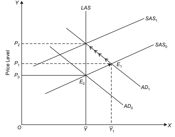
• Suppose the government increases expenditure without raising taxes and finances it by borrowing from the central bank, which creates new money; this increases money supply and shifts aggregate demand rightward from \(AD_0\) to \(AD_1\).

• The new aggregate demand curve \(AD_1\) intersects the short-run aggregate supply curve \(SAS_0\) at point \(E_1\), raising price level from \(P_0\) to \(P_1)\) and real GDP from \(\overline{Y}\) to \(Y_1\).

• The rise in price level occurs because aggregate demand increases more than aggregate supply, creating demand–supply imbalance; since (SAS) is upward sloping (not horizontal), output rises only partially while prices increase significantly.

• In the short run, money wage rate (W) is assumed constant; therefore, when price level rises \((P_1 > P_0)\), real wage falls:
  $$\text{Real Wage} = \frac{W}{P}$$
  so \(\frac{W}{P_1} < \frac{W}{P_0}\).

• The fall in real wage and output beyond potential level \((Y_1 > \overline{Y})\) reduces unemployment below the natural rate, creating excess demand for labour and putting upward pressure on money wages.

• Workers demand higher wages to restore lost purchasing power; as firms raise wages, production costs increase, causing the short-run aggregate supply curve to shift upward (leftward) from \(SAS_0) toward (SAS_1\).

• This wage–price adjustment continues until the new short-run aggregate supply curve intersects \(AD_1\) at point \(E_2\) on the long-run aggregate supply (LAS) curve, restoring output to potential level \(\overline{Y}\) but raising price level further to \(P_2\).

• At the new long-run equilibrium \(E_2\):
  $$Y = \overline{Y}, \quad P = P_2$$
  and money wage rises proportionately with price level, so real wage is restored:
  $$\frac{W_2}{P_2} = \frac{W_0}{P_0}.$$

• The movement from \(E_1\) to \(E_2\) occurs gradually through successive wage adjustments and upward shifts of the short-run aggregate supply curve, ultimately leaving real GDP unchanged at potential level but with a permanently higher price level, illustrating demand-pull inflation in the long run.