Market Structures, Competitive and Non-Competitive Equilibria and their Efficiency Properties – Notes

Introduction

A Market is a place where the exchange of goods takes place. The market is the nervous system of modern economic life where producers and consumers carry out the sale and purchase transactions. The market has a different and wider meaning in economics, as it does not refer to a specific place. In Economics, a Market is a region where the buyers and sellers don’t have to assemble at a specific place for the sale and purchase of goods. Instead, they have to be in contact with each other through any communication means, such as the internet, letters, mail, telephone, etc. 

Market refers to the whole region where buyers and sellers of a commodity are in contact with each other for the purchase and sale of the commodity. 

• Markets can exhibit different structures based on the number of buyers and sellers and the degree of competition. Common structures include perfect competition, monopolistic competition, oligopoly, and monopoly.
• Markets are driven by the forces of supply and demand. Sellers provide goods or services, while buyers demand them.
• In a competitive market, equilibrium occurs when the quantity supplied equals the quantity demanded at a specific price, known as the equilibrium price.
• Markets are considered efficient when they allocate resources to their most valued uses.

Essentials or Characteristics of a Market

1. Area: In economics, a market is not related to a specific place, instead, it spreads over an area that becomes the point of contact between the producers/sellers and consumers/buyers. With the advancement of technology and modern means of communication, the market area of a product has become wide. 
2. Commodity: In economics, a market is not related to a specific place but to a specific product. It means that a market can exist if there is one commodity that will be purchased and sold among the buyers/consumers and sellers/producers. 
3. Buyers and Sellers: Another characteristic of a market is the presence of buyers and sellers. The buyers and sellers must contact each other in the market. However, it does not mean that they should meet physically, the contact can be through modern means of communication, like the internet, mail, telephone, etc. 
4. Competition: For a market to exist, it is necessary that there is free competition amongst the buyers and sellers. The absence of competition in the market results in the charging of different prices for the homogeneous commodity by the sellers. 

Market Structure

The number and types of firms operating in the industry and the nature and degree of competition in the market for the goods and services is known as Market Structure. To study and analyze the nature of different forms of market and issues faced by them while buying and selling goods and services, economists have classified the market in different ways. 

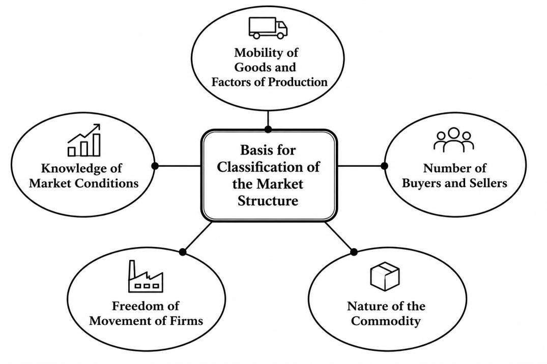
Basis for Classification of the Market Structure

The factors determining the market structure are as follows:

1. Number of Buyers and Sellers: The volume/number of buyers and sellers in the market of a commodity exercises a great influence on the price of a commodity. If there are a large number of buyers and sellers in the market, then a single buyer or seller cannot influence the price of a commodity. However, if there is one seller of a commodity, such as Railways, then the seller has great control over its price. 
2. Nature of the Commodity: The nature of the commodity has a great impact on the price of the commodity. If a commodity is homogeneous in nature (identical goods such as pen, paper, etc.), then it is sold at a uniform price in the market. If a commodity is heterogeneous in nature (non-identical, totally different goods, such as different toothpaste brands, etc.), then it may be sold at different prices. However, commodities with no close substitutes, such as Railways can charge a higher price from the buyers. 
3. Freedom of Movement of Firms: Freedom in entry and exit of firms results in price stability in the market. However, restrictions on the entry of new firms or exit of the existing ones can lead to the firms influencing the price of goods and services, as they have no fear of competition from other existing or new firms. 
4. Knowledge of Market Conditions: If the buyers and sellers are aware of the market conditions and have full knowledge about them, then the uniform price of goods and services prevails in the market. Whereas, if the buyers and sellers are unaware of the market conditions, then sellers are in a position to charge their customers different prices. 
5. Mobility of Goods and Factors of Production: Free movement of factors of production from one place to another results in a uniform price in the market. However, if the movement of factors of production is not free, then the prices may differ from each other. 

Forms of Market Structure

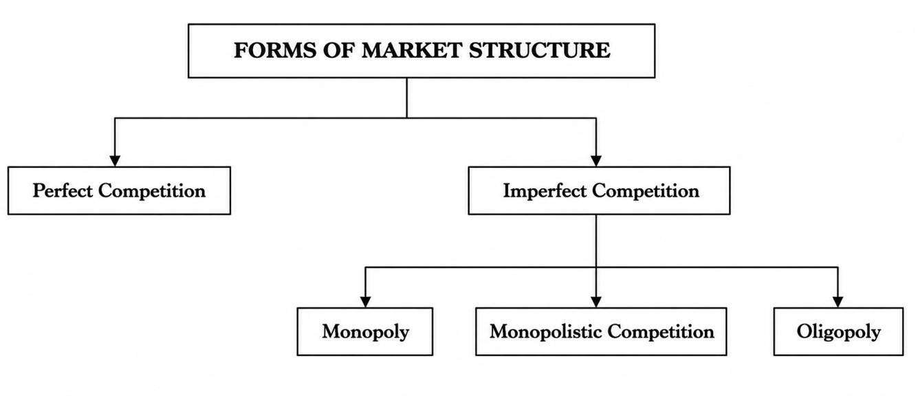
The different forms of market structure are Perfect Competition and Imperfect Competition (Monopoly, Monopolistic Competition, and Oligopoly). 

Perfect Competition

A market situation where a large number of buyers and sellers deal in a homogeneous product at a fixed price set by the market is known as Perfect Competition. Homogeneous goods are goods of similar shape, size, quality, etc. In other words, in a perfect competitive market, the sellers sell homogeneous products at a fixed price determined by the industry, not by a single firm. In the real world, the situation of perfect competition does not exist; however, the closest example of a perfect competition market is agricultural goods sold by the farmers. Goods like wheat, sugarcane, etc., are homogeneous in nature and their price is influenced by the market. 

Key Features:

The key features of perfect competition include a large number of sellers, identical products, perfect knowledge, and zero entry barriers.

• Sellers/Buyers: Very many small firms & buyers
• Product: Homogeneous (identical)
• Price Power: Price taker (P = MR = AR)
• Entry/Exit: Free, negligible barriers
• Information: Perfect information
• Profit: Supernormal profit only in short run; normal profit in long run
• Efficiency: Allocative & productive efficiency in long run
• Examples: Agricultural markets, commodity exchanges

Advantages:

• Cheap Prices to Consumers: Very, very strong competition results in market price being very low under no set pricing capability by firms, benefiting consumers.
• Resource Efficiency: In fact, firms are required to operate and get it within the point when price equals marginal cost (P = MC); afterward, it will generate allocative efficiency.
• Free Entry and Exit: Firms can freely enter or leave the market such that it exists as dynamic and flexible to demand changes.
• Consumer Sovereignty: Firms have no power on the price and all depend on consumer needs.

Disadvantages:

All the developments were made just for theorization because there are no profits in the long term, and products are homogeneous, so companies have no incentive to innovate or improve themselves for the simple reason there are no real profits built-in.

• Margins Are Really Thin: Keeping competitive forces firms on very little profits that are not going to last.
• No choice of product: All products are uniform; therefore, no choices in brand names, quality, or features are available to the consumers.
• Not Realistic in Today’s Markets: True perfect competition is rare in today’s condition; it is true that the most markets do not show any kind of differentiation or control.

Monopoly

Monopoly is a completely opposite form of market and is derived from two Greek words, Monos (meaning single) and Polus (Meaning seller). A market situation where there is only one seller in the market selling a product with no close substitutes is known as Monopoly. For example, Indian Railways. In a monopoly market, there are various restrictions on the entry of new firms and exit of the existing firms. Also, there are chances of Price Discrimination in a Monopoly market. 

Key Features:

Characteristics of monopoly include price-making power, lack of close substitutes, high entry barriers, and long-run supernormal profits.

• Sellers/Buyers: Single seller, many buyers
• Product: Unique, no close substitutes
• Price Power: Price maker (sets P where MR = MC)
• Entry/Exit: Very high barriers (legal, tech, natural monopoly)
• Demand: Faces market demand (downward sloping)
• Profit: Can sustain long-run supernormal profits
• Efficiency: Deadweight loss, allocative inefficiency (P > MC)
• Examples: Natural utilities, railways (regulated)

Advantages:

• Uniform Quality and Service: Since there is no competition at all, the firm can provide constant delivery of goods and services. 
• Heavy R&D Investment: Monopolies are free to spend much of their income on R&D due to the guaranteed profits in most cases, more than usually in the technology and medicine sectors. 
• Economies of Scale: Monopoly firms can produce at a lower average cost, particularly in industries like utilities or railways.
• Natural Monopoly: Natural monopolies can be useful in such industries as the one that deals with electricty and water supply since they do not necessitate duplication of infrastructures.

Disadvantages:

• High Prices and Low Output: Ultimately, without competition, they may restrict their supply in order to raise their prices and leave consumers worse off. 
• Consumer Exploitation: There are no alternatives readily available to consumers which makes it impossible to reject the firm’s pricing and service conditions. 
• Lack of interest in Improvement and Innovation: Lack of competition pressure may make the firm become dysfunctional and degenerate in terms of sorting improvements over time. 
• Efficiency Losses and Deadweight Losses: Monopolies operate where marginal cost is less than price (P > MC), causing welfare loss to society.

Monopolistic Competition

A Monopolistic Competition Market consists of the features of both Perfect Competition and a Monopoly Market. A market situation in which there is a large number of firms selling closely related products that can be differentiated is known as Monopolistic Competition. The products of monopolistic competition include toothpaste, shampoo, soap, etc. For example, the market for soap enjoys full competition from different brands and has freedom of entry showing the features of a perfect competition market. However, every soap has its own different feature, which allows the firms to charge a different price for them. It shows the features of a Monopoly Market.

Key Features:

• Sellers/Buyers: Many firms, many buyers
• Product: Differentiated (branding, features)
• Price Power: Some control due to differentiation (AR > MR)
• Entry/Exit: Relatively easy (low–moderate barriers)
• Competition: Heavy non-price competition (ads, design, service)
• Profit: Short-run supernormal; long-run normal (entry erodes profits)
• Efficiency: Excess capacity, not fully efficient
• Examples: Restaurants, apparel, toothpaste

Advantages:

• Variety of Products: Consumers enjoy a variety of almost similar, but differentiated products (for example: different types of coffee shops).
• Branding and Innovation Stimulated: Firms invest in product design, client experience, and branding for that wow factor.
• High Consumers’ Choice: Consumers have several options according to individual preferences on price, quality, or brand loyalty.
• Ease to Enter/Exit: Similar to perfect competition, there are low barriers to entry, thus making new entry easy for new firms entering the market.

Disadvantages:

• Higher Prices Relating to Perfect Competition: Differentiation and branding allow firms to exercise some degree of price-power, hence inflate prices somewhat.
• Excess Capacity and Inefficiency: Under-differentiated demand and under-utilized resources imply that firms do not necessarily produce at least cost. 
• High Costs of Marketing and Advertising: Promotion becomes necessary, and those costs are often passed on to consumers.
• Only Profits in Short Run: In the long run profit decreases with competition in the market. Therefore, firms have to struggle to keep surviving profitably.

Oligopoly

A market situation where the number of big sellers of a commodity is less and the number of buyers is more is known as Oligopoly Market. As the number of sellers in this market is less, the price and output decision of one seller impacts the price and output decision of other sellers in the market. In other words, the interdependence among the sellers of a commodity is high. For example, luxury car producers like BMW, Audi, Ford, etc., come under Oligopoly Market, as the number of sellers of luxury cars is less and its buyers are more.

Key Features:

• Sellers/Buyers: Few large firms dominate (2–10)
• Product: Homogeneous or differentiated
• Price Power: Significant, but interdependent decisions
• Entry/Exit: High barriers (scale, brand, regulation)
• Behavior: Kinked demand, price rigidity; risk of collusion/cartels
• Profit: Can sustain supernormal profits
• Efficiency: Mixed; can have economies of scale but risk welfare loss
• Examples: Telecom, airlines, autos

Advantages:

• Economies of Scale: Unlike small firms, big firms enjoy lower average costs because of mass production, ensuring lower market prices if passed to consumers.
• Increase in Innovation through Competitive Pressure: Rivalry among few firms often ignites improvements in products and technological innovation.
• Stable Price: Because they all fear price wars, they discourage instabilities in price changes, thus creating a stable market for consumers.
• Heavy Investment in R&D: Their profits accrue for further investment in research resulting to quality products and technological innovation in the long run.

Disadvantages:

• Price Collusion: Firms may unofficially agree to keep prices high (cartel behavior), which harms consumers.
• High Barriers to Entry: Massive start-up costs, brand loyalty, and economies of scale make it difficult for new firms to break into the market.
• Misleading Non-price Competition: A heavy advertising campaign creates artificial differences rather than real product improvement.
• Consumer Exploitation Possible: If firms act like a cartel, prices can stay artificially high with limited alternatives. 

Competitive Equilibrium

• A Competitive Equilibrium is a market situation in which buyers and sellers interact under perfect competition, and the equilibrium price and quantity are determined solely by the forces of demand and supply. In this market structure, individual buyers and sellers are price takers, meaning that no single participant has the power to influence the market price.
• Competitive equilibrium occurs when the quantity demanded equals the quantity supplied.

$$Q_D = Q_S$$

​

• At this equilibrium price, there is neither excess demand nor excess supply. Consumers purchase the quantity they desire, producers sell all the output they wish to produce, and the market clears automatically.
• The concept of competitive equilibrium is closely associated with the work of Léon Walras, who developed the theory of General Equilibrium, explaining how all markets in an economy simultaneously reach equilibrium through price adjustments.

Perfectly Competitive Market

• The important characteristics of the perfectly competitive market are:

  • (i) There are a large number of sellers (firms) and buyers (consumers) in the market.

  • (ii) Firms are producing homogenous products.

  • (iii) The firms are free to enter or exit the industry.

  • (iv) The factors of production are completely free to move from one firm to another firm.

  • (v) All sellers and buyers have complete knowledge of the conditions of the market.

• These are some important attributes of perfect competition. The price of the product remains the same throughout the market. The firm is a price taker and its demand curve is infinitely elastic. That is, the demand curve is a horizontal line. The demand curve of the individual firm is also its average revenue as well as marginal revenue curve. The cost structure such as average cost (AC) and marginal cost (MC) are as usual.

• Under the above assumptions/conditions, the equilibrium situation of the firm and industry operating under perfect competition in the short run and long run will be discussed here. The objective of the firm is profit maximization. The effects of changes in costs, imposition of a tax, or providing subsidy by the government on the equilibrium condition will be given in different subsections. Derivation of the supply curve of the firm and industry will also be discussed in a subsection.

Equilibrium of Firm in Short Run:

• Firms are the producing units of various products. The objective of all the firms is profit maximization. A firm remains in equilibrium where it attains the maximum profit and produces the optimum level of output. Under a perfectly competitive market, the condition for the equilibrium of a firm is that “the marginal cost (MC) should be equal to the marginal revenue (MR)” i.e.;

$$MC = MR$$

$$MC = P_y \; (MR = P_y \text{ in the perfect competition})$$

• At this point, profit is the maximum and optimum level of output produced.

• If MC < MR, Total profit has not been maximized and the profit is increased by expanding output.

$$MC < MR$$

• If MC > MR, Total profit/loss is being reduced by reducing production.

$$MC > MR$$

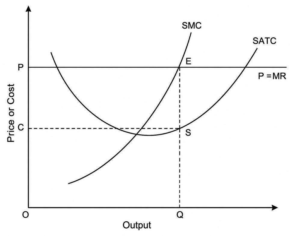
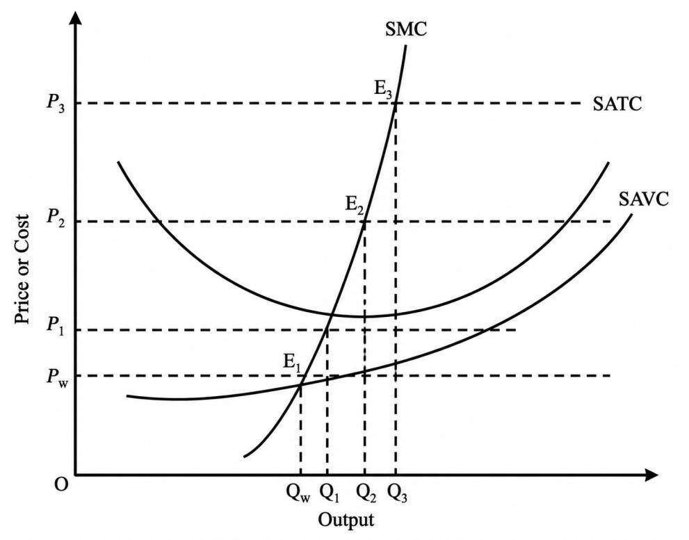
• This may be illustrated with the help of Figure 5.1. We draw the SATC and SMC of the firm. In perfect competition, the demand curve of the individual firm is the horizontal line. The demand curve which is also the MR and price line in this market is drawn. In the figure, the firm is in equilibrium at the point ‘E’ where the SMC curve cuts the MR or price line from below.

• At the equilibrium condition, the firm is producing an optimum level of output Q at price ‘P’ and is having the maximum profit. The second-order condition for equilibrium requires that the SMC curve has a rising trend at the point of intersection with the MR curve. It means that the SMC curve must cut the MR curve from below.

• In the figure, you will find that the total revenue of the firm is equal to the area POQE and the total cost is equal to the area COQS. Thus total profit will be equal to the area PCSE.

• The firm mostly earns excess profit in the short run. But it is not necessary that the firm always earn excess profit. It depends on the level of the SATC and the price of the output. In the short run, the firm will continue to produce only if it covers its variable costs, otherwise, it will close down. The point at which the firm just covers its variable cost is called the closing down point \(P_w\) (Fig. 3). At this point, the SAVC is just equal to the price of output. If the price falls below \(P_w\), the firm will not produce at all.

• Mathematically, we can also work out the optimum level of output, if we know the cost function and the price of output. Find out the MC from the given cost function and equate MC to the price of output. We solve this equation for output ‘Q’ which is the optimum level of output to be produced at the equilibrium condition of the firm.

Supply Curve of Firm and Industry:

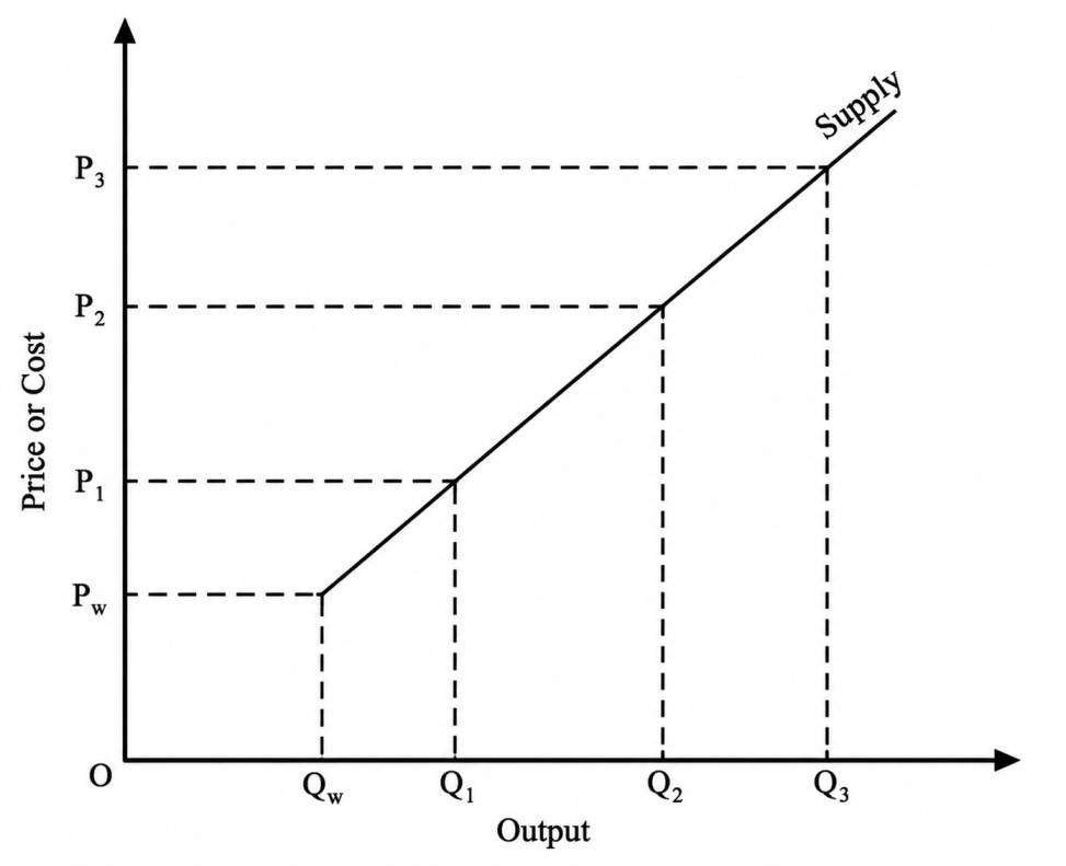
• The short-run supply curve of a firm under perfect competition is derived by different points of intersection of SMC curve and price line (Fig. 4). As the price of output changes, the quantity supplied by the firm changes. As the price rises, the output supplied by the firm increases. The price line intersects the SMC curve above the minimum average variable cost. If the price falls, the quantity supplied decreases. The firm will supply up to the minimum SAVC or up to \(P_w\) point but the firm will not supply if the price falls below \(P_w\). Because at a lower price the firm does not cover its short-run average variable cost.

• If we plot different points of intersection of the MC curve and price line on a separate graph (Fig. 5) we get the short-run supply curve of the individual firm. This supply curve of the firm is identical to its MC curve to the right above the minimum SAVC or closing down point, \(P_w\). Below \(P_w\) the quantity supplied by the firm is zero. The supply curve of the firm as shown in Fig. 5 is a straight line with a positive slope.

• The industry-supply curve is the horizontal summation of the supply of the individual firms in the industry. That is, under the conditions if all factors like technology and price of inputs remain constant, the total supply of a commodity of the industry at each price is the sum of the quantity of commodity supplied by all the firms in the industry at that price.

Equilibrium of Firm in Long Run:

• In the long run, all the inputs are variable. An entrepreneur has the option of the adjustment of the plant size as well as output level to achieve maximum profit. The condition for the long-run equilibrium of the firm is that the long-run marginal cost should be equal to the long-run average cost and also equal to the output price i.e.;

$$LMC = LAC = P$$

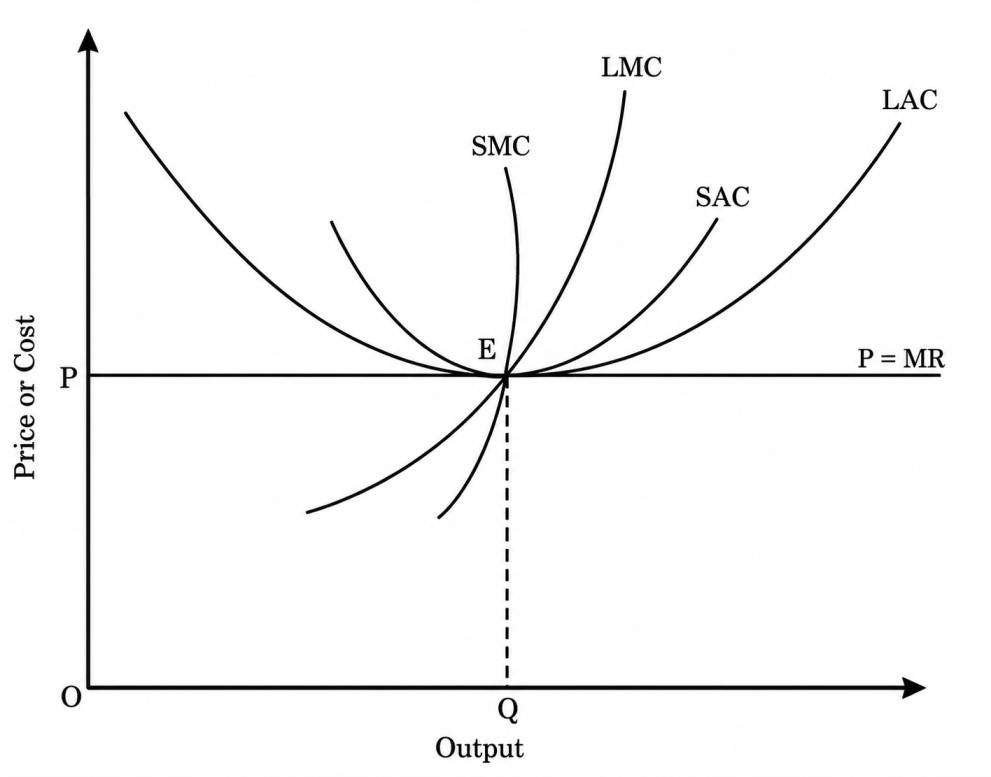
• In the long run, the firm does not earn excess profit. It earns just normal profit. The firm adjusts its plant size and produces the output level at which LAC is the minimum possible. Hence at equilibrium, the LMC is equal to the SMC and LAC is equal to the short-run average cost (SAC). Thus the equilibrium condition is:

$$LMC = LAC = SMC = SAC = P = MR$$

• This condition is presented in Fig. 6. In the figure, you can see that the firm produces the quantity Q at price P and gets the normal profit.

Effects of Changes in Costs on Equilibrium:

• As a result of an increase in the fixed costs, AFC and ATC curves will shift upwards. However, the AVC and MC curves will not be affected. Thus the equilibrium position of the firm is not affected in the short run. Hence, the output level and the price will not change in the short run due to a change in the fixed costs.

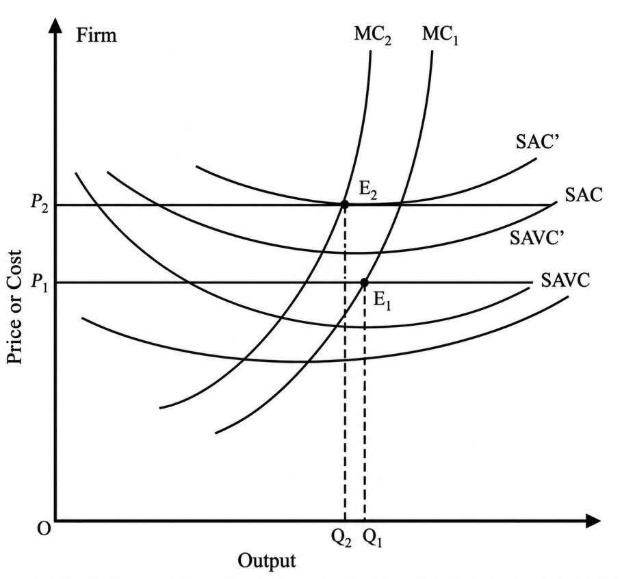
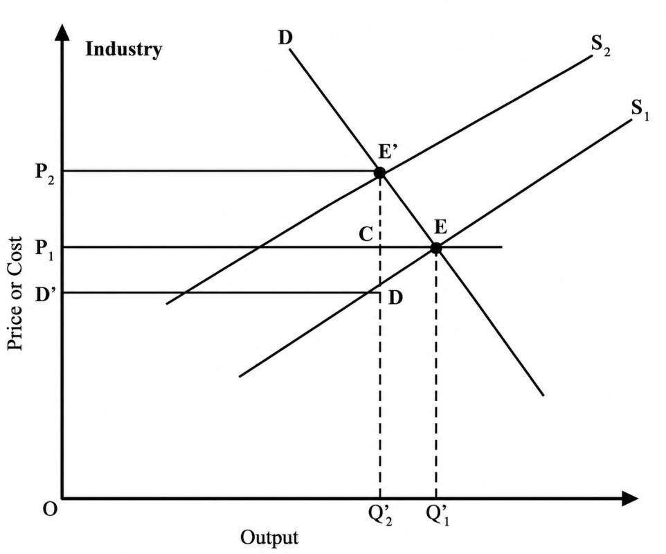
• If the variable costs increase, the AVC, AC, and MC curves of the firm shift upwards to the left (Fig. 7). The equilibrium of the firm changes due to changes in the marginal costs. As a result of the increase in the average variable costs, the quantity supplied by the firm at the going market price will decrease.

• Thus, even in the short run, the market supply will shift upwards to the left. Hence, at market demand, the price will rise due to declining market supply (Fig. 8).

Effects of Imposition of Tax on Equilibrium:

• As a result of the imposition of a lump sum tax or profit tax by the government, in the short run, the equilibrium of the firm will not change. Hence, the output level and the price will not change but the total profits of the firm will reduce.

• Sometimes Government imposes a specific sales tax, that is, tax per unit of output produced. Such rising tax causes a shift of the AC and MC curves upwards to the left. Due to the shift of the MC curve to the upward, the supply of firms will reduce (Fig. 7). The price will increase because of decreasing market supply (Fig. 8).

• How much price will increase? Will the price rise be equal, smaller, or greater than the specific tax? It depends on the price elasticity of supply at the given market demand. More is the price elasticity of supply; a greater tax burden is to be borne by the consumer. Hence, the price will raise more.

Effects of Providing Subsidy on Equilibrium:

• In order to encourage production, the government provides a subsidy to the producers. Assuming government gives some subsidy on the per unit of output, it will affect the cost. The cost per unit of output will decrease. Hence the AC and MC shift downwards (Fig. 9). Due to the shift in the MC curve to the lower side, the supply of the firm will increase and the price will decrease.

• The price will decrease due to market supply increases (Fig. 10). How much price will reduce? It depends on the price elasticity of supply at the market demand.

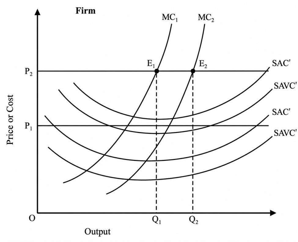
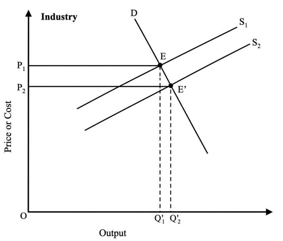
Fig 10. Changes in Supply

Non-Competitive Equilibrium

Monopoly Market

• A monopoly is a market structure in which there is only one seller (producer) of a commodity. There are no rivals in the market. There is no close substitute for the commodity produced. There are barriers to entry for the firms.

• Some important points of the monopoly are as follows: In a monopoly, the demand curve is negatively sloped which is identical to the market demand curve. The marginal revenue curve is also having a negative slope. Furthermore, marginal revenue is less than the price at all the points. The relationship between MR and P is given as:

$$MR = P\left(1 – \frac{1}{e}\right)$$

• where (e) = price elasticity of demand.

• The monopolist can change both the price and output level. He has the market power to change the price or output level of the commodity produced in the market. In order to increase the sale of a product, he can reduce the price of the product. The goal of the monopolist is profit maximization. He is able to change the price or output level for attaining maximum profit.

• The cost structure of the monopolist is identical to the perfectly competitive firm. The equilibrium condition under monopoly in the short run and long run and its applications are discussed in the following sub-sections.

Equilibrium of Monopolist in Short Run:

• The short-run equilibrium of the firm under monopoly is at the point where the monopolist attains the maximum profit. The condition for profit maximization of the firm under monopoly is that the marginal cost (MC) should be equal to the marginal revenue (MR) i.e.;

$$MC = MR$$

• The equilibrium condition of the firm in the short run is given in Fig. 11. You will find in the figure that the MC curve intersects the MR curve at point ‘E’. The second-order condition for the equilibrium of the firm requires that the MC curve intersects the MR curve from below. This you can see in the figure. At this point, the monopolist produces the optimum quantity of output ‘Q’ at the price ‘P’. The cost of production is ‘C’. It is to be noted that the price is higher than the marginal revenue. The monopolist earns the excess profit which is equal to the area APCB. The profit and loss of the monopolist depend upon the price and average total costs.

• The monopolist can either set his price and sells the quantity of product in the market or produces an output level and sells at a price. Thus, the monopolist cannot decide independently both the price and the quantity of output to produce.

• Mathematically, we can also find out the optimum quantity of output if the cost function and demand function are given. From the cost function, you can find out the MC function. The total revenue function which is equal to ‘PQ’ is worked out from the demand function. From the total revenue function, you can work out the MR function. Apply the condition of MC equals MR for equilibrium. Solve this relation for a quantity of output ‘Q’. Find out the price from the demand function by putting the value of quantity ‘Q’.

• It is important to mention here that the change in variable costs, imposition of sales tax, providing subsidies, and shift in the market demand will affect the equilibrium of a firm in monopoly. If variable cost increases, the supply will decrease and the price will increase because of an upward shift in the MC curve as you have seen in the case of the perfectly competitive market. A similar effect of the imposition of sales tax on the quantity supplied and the price will be observed. As a result of providing subsidies, the supply of output will increase and the price will reduce. If market demand shifts, either way, the equilibrium of the firm changes. Consequently, the quantity supplied and the price will change.

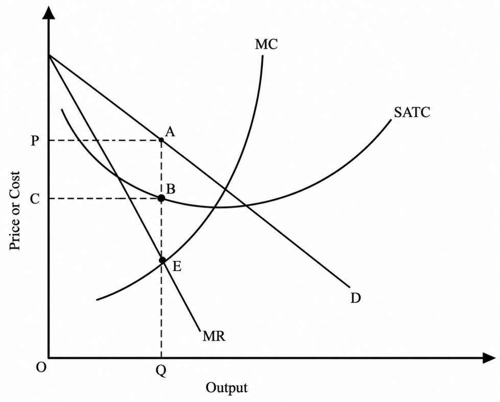
Fig 11. Equilibrium of Monopolist in Short Run

Supply of Monopolist:

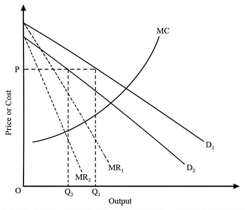
• There is no unique relationship between price and quantity supplied in the case of a monopoly market. The same quantity may be supplied at different prices depending on market demand. Graphically, this is shown in Fig. 12. The quantity ‘Q’ will be supplied at price
  $P_1$

   

  ​ if demand is $D_1$

   

  , while the same quantity ‘Q’ will be supplied at price $P_2$

   

  ​ if demand is $D_2$

   

  ​.
• Similarly, for a given MC of the monopolist, different quantities may be supplied at one price, depending upon the market demand and the corresponding MR curve. This situation is depicted in Fig. 13. Given the MC of the monopolist, he would supply
  $Q_1$

   

  ​ at price $P$

   

  if the market demand is $D_1$

   

  ​ while at the same price $P$

   

  , he would supply only $Q_2$

   

  ​ if the market demand is $D_2$

   

  .

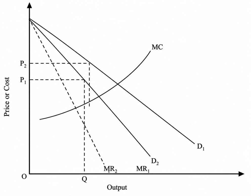
Fig 12. Supply of Monopolist

Equilibrium of Monopolist in Long Run:

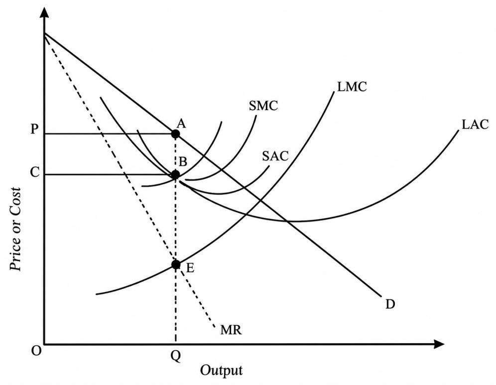
• In the long run, the monopolist has the time to expand his plant. With entry blocked, it is not necessary for the monopolist to reach up to the optimum plant. He may also build sub-optimal plant and earns supernormal profits even in the long run.

• Let us consider a case where the monopolist is using sub-optimal plant size (Fig. 14). The condition for equilibrium, in the long run, is that the long-run marginal cost (LMC) should be equal to the marginal revenue i.e.;

\(LMC = MR\)

• The equilibrium is at point ‘E’ where the price is P and the quantity is Q. The long-run profit is given by the area PCBA. Consider the firm is adopting a sub-optimal plant size, the SAC is tangent to the LAC at its falling part (less than minimum LAC) and also SMC is equal to the LMC i.e.;

\(SMC = LMC = MR\)

• Since the monopolist is not using the optimum plant size where LAC is not the minimum one, there exists excess capacity.

Price Discriminating Monopolist:

• Price discrimination exists when a producer sells the same product at different prices in different markets. Price discrimination is easily implemented by a monopolist because he has control over the whole supply of a commodity. A monopolist can sell the same product to the poor and rich people at different prices and considers the welfare of the society. In this way, he is able to increase the total profit.

• There are some necessary conditions for the implementation of price discrimination:

  • (a) Different price elasticities of demand in the various markets.

  • (b) Spatially separated markets – no reselling takes place.

• The objective of the monopolist is profit maximization. He would like to know how much to sell in each market at what price so that the total profit is the maximum. The MR in each market is different due to the different demand curves of the market. The profit in each market is maximized by equating the MR of each market to the MC as a whole product i.e.;

$$MR_1 = MC$$

First market

$$MR_2 = MC$$

Second Market

• That is,

$$MC = MR_1 = MR_2$$

• This is the condition for profit maximization of the price discriminating monopolist.

• If,

$$MR_1 > MR_2$$

• The monopolist will sell more quantity in the first market and less quantity in the secondary market until the condition of \(MR_1 = MR_2\) is fulfilled.

• Graphically, the discrimination of the prices and quantities in the two markets is shown in Fig. 15. The total quantity is produced where the aggregate MC and the MR intersect with each other at point ‘E’. Thus, the total quantity produced is OX at a uniform price P. Now we draw a line ‘ER’ parallel to the quantity axis. This line cuts the \(MR_1\) at point \(E_1\) and the \(MR_2\) at point \(E_2\). At these points we have the required condition i.e.;

\(MC = MR_1 = MR_2\)

• From \(E_1\) and \(E_2\) we drop vertical lines to the quantity axis and we extend them upwards up to the demand curves \(D_1)\) and \(D_2\) in two markets. These vertical lines define the quantity and price in each market. Thus in the first market, the monopolist will sell \(OX_1\) at the price \(P_1\) and in the second market, the monopolist will sell \(OX_2\) at the price \(P_2\). So the total output is:

\(OX = OX_1 + OX_2\)

• The profits from price discrimination are more than selling the whole output at a uniform price P. This is known as third-degree price discrimination.

• If the MRs are equal in two markets, it does not necessarily imply the equality of price in two markets. It depends on the price elasticity of demand in the markets. With the relationship between MR and price as given earlier, you can find out the price in each market if the demand elasticity of each market is known.

• It is to be noted that the price is lower in the market where the price elasticity of demand is greater and vice-versa. For the same product, the monopolist charges the lower price from the poor society where the price elasticity of demand is greater and charges the higher price from the rich society where the price elasticity of demand is lower. In this way, monopolist takes into consideration social welfare. One of the effects of price discrimination is that the monopolist manages to reap part of the consumer’s surplus and thus increases his total revenue.

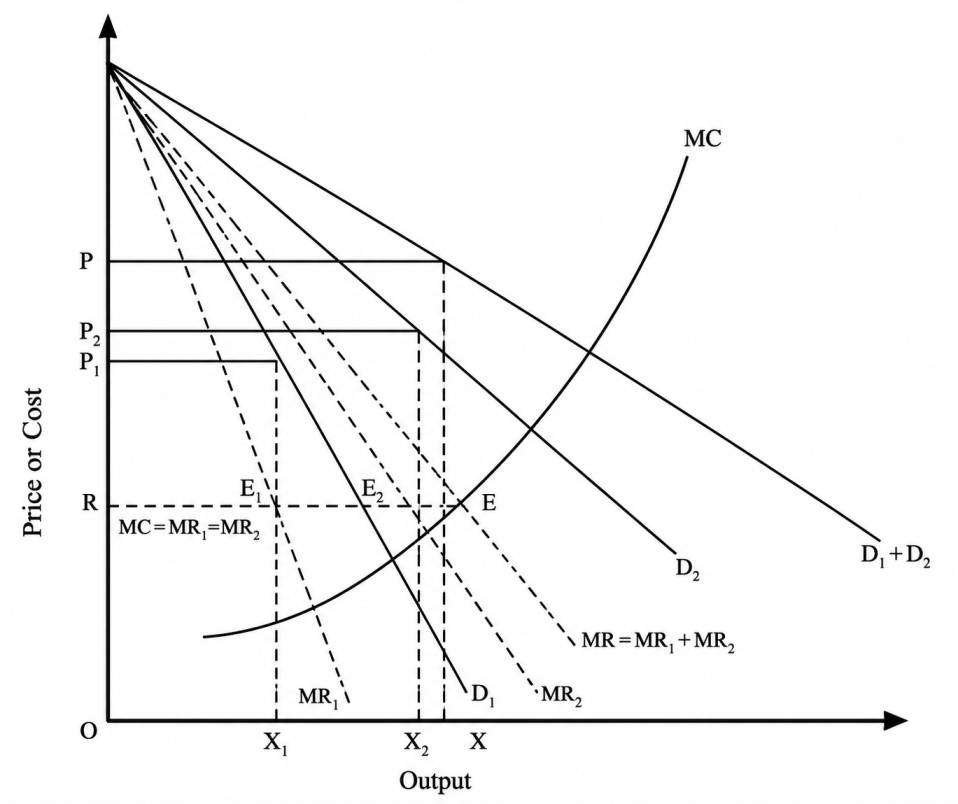
Fig 15. Price Discriminating Monopolist

Regulation of Monopoly Price by Government:

• In the case of a simple monopoly, the equilibrium price is P and the quantity is Q which is attained by the equilibrium condition as:

$$MC = MR$$

• Under this situation, the monopolist earns the excess profit by charging higher prices P. But sometimes government makes interventions and regulates the monopoly prices which are allowed to charge by the private monopolist. The government has to set the prices or different levels of price by adopting a price discriminating policy.

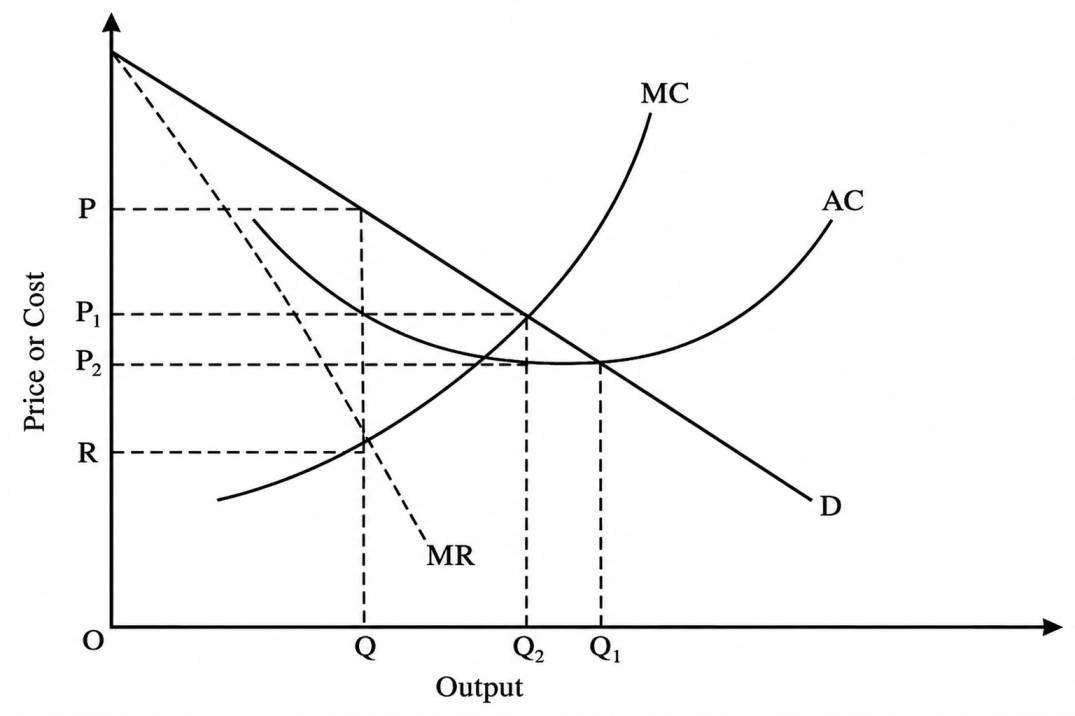
• Firstly, the government may set a price at the level of MC. That is, the MC equals to price i.e.;

$$MC = P_1$$

• This you can see in Fig. 16. The price is \(P_1\) which is lower than the equilibrium price P and output level \(Q_1\) is higher than the equilibrium quantity Q of the product. There is still profit to the monopolist.

• Secondly, the government may set a price equal to AC, i.e.;

$$AC = P_2$$

• In Fig. 16, the price is \(P_2\) which is lower than the equilibrium price P and it leads to higher output \(Q_2\) in comparison to equilibrium output Q. Although the price is lower than the equilibrium price P, the monopolist still gets normal profits.

• Sometimes the government may apply a price discrimination scheme for social welfare, particularly in public utilities like electricity, gas, telephone, railways, etc. Government charges the different prices from different sections of the society or on the basis of the levels of consumption of the utility goods/services.

Monopolistic Competition

• So far as we have discussed two important markets namely perfect competition and monopoly. These markets are at two extremes from the point of view of a number of producers. In a perfectly competitive market, there is a large number of producers producing homogenous products, whereas in a monopoly market there is only one producer. In the case of the monopolistic competitive market, there is a large number of firms that are producing heterogeneous products. The products are slightly differentiated yet they are close substitutes for one another. Product differentiation is an important feature of this market.

• Monopolistic competition contains some elements of both perfect competition and monopoly. Perfect competition is in the sense that there is a sufficiently large number of producers so that the actions of a producer have no perceptible influence upon his competitors. The market is like a monopoly in the sense that when products are differentiated in nature, then each product is unique and its producer has some degree of monopoly power.

• Chamberlin has developed a model of monopolistic competition. In place of industry, he has given the concept of ‘large group’ which is the collection of a large number of firms producing very closely related products. For example, there is a large number of firms producing soap of different brands which are the substitute for one another.

• Chamberlin has given the following assumptions/characteristics of monopolistic competition for the large group model:

  1. There is a large number of sellers (producers) and buyers in the group.

  2. The products of the sellers are differentiated, yet they are close substitutes for one another.

  3. There is free entry and exit of firms in the group.

  4. The prices of factors of production and technology are given.

  5. Finally, Chamberlin makes the ‘heroic’ assumption that both demand and cost curves for all products are uniform/identical throughout the group. Although this assumption is unrealistic. But for simple analysis, it has been assumed.

• The goal of the firms in the product group is profit maximization both in the short run and long run. Chamberlin adopted that the shape of cost curves is similar to the traditional theory of the firm. The AVC, ATC, and MC are similar to that of perfect competition and are worked out assuming only a single level of output.

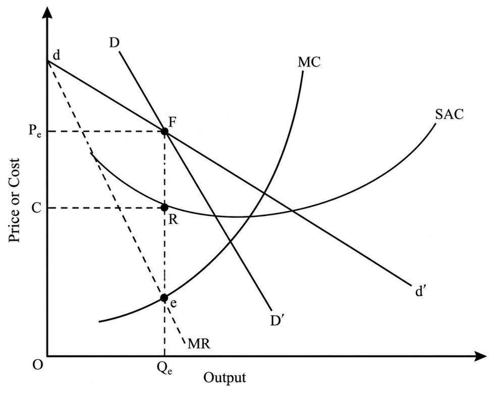
• Because of the product differentiation, the producer has some discretion in the determination of price. He is a price taker but has some degree of monopoly power that he can exploit. Thus the individual firm possesses a negatively sloped demand curve (dd’) for its distinct product. In monopolistic competition, there is one more demand curve (DD’) which is known as the actual sales curve or the share of the market curve or the effective demand curve. (DD’) demand curve shows the actual sales of the firm at each price after accounting for the adjustments of the prices of the other firms in the ‘product group’. The (DD’) demand curve is less elastic than that of the (dd’) demand curve. That is (DD’) demand curve is steeper than the (dd’) demand curve because the actual sales from a reduction in price are smaller than expected on the basis of the (dd’) demand curve as all firms reduce their price and expand their own sales simultaneously.

Equilibrium of Firm in Short Run:

• Chamberlin said that the short-run equilibrium of a firm in monopolistic competition acts as a monopoly. According to Chamberlin the cost and demand curves are identical for all the firms in the product group under monopolistic competition. In the short run firm maximizes its profit by producing the output at which marginal cost is equal to the marginal revenue, i.e.,

$$MC = MR$$

• The price in the market will be the same. No firm has an incentive to change its own price. The second condition for profit maximization requires that the MC cuts the MR from below.

• The equilibrium of a firm in the short run is illustrated in Fig. 17. In the figure, MC and SAC curves are drawn. The individual firm’s demand curve is presented by (dd’) and the share of the market demand curve is shown by (DD’). For the firm’s demand curve (dd’), the MR curve is also drawn. The firm is in equilibrium at the point ‘e’ when the MC curve intersects the MR curve. We extend the vertical line passing through the equilibrium point ‘e’ and it meets the demand curve (dd’) at ‘F’ where the demand curve (dd’) intersects the share of the market demand curve (DD’). The firm produces the quantity \(Q_e\) at the price \(P_e\). In the short run, the firm earns an abnormal profit which is equal to the area PFCR.

Equilibrium of Firm in Long Run:

• As you have seen in the case of short-run equilibrium, the firm realizes the abnormal profits. In the short run, the existing firms do not have any incentive to adjust the price but in the long run, the existing firms are in a position of price adjustment. Secondly, in the long run, new firms also enter the product group because of the attraction of excess profits. Hence Chamberlin gave two models for the long-run equilibrium of a firm:

1. 1. Long-run Equilibrium of Firm with Price Competition.
   2. Long-run Equilibrium of Firm with Price Competition and Free Entry of Firms.

1. Long-run Equilibrium of Firm with Price Competition:

• In this model, it is assumed that there are optimum numbers of firms in the product group. Neither entry nor exit will be taken place by the firms in the product group. The ruling price in the short run is assumed to be higher than the equilibrium price. In this model, Chamberlin assumed also that the long-run cost structure and demand curve are identical for all the firms in the product group. The price adjustments are shown along the (dd’) demand curve. The actual sales of the firm at each price after accounting for the adjustments of the prices are shown by actual sales or share of the market demand curve (DD’).

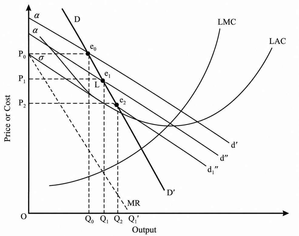
• We assume that the firm is at the non-equilibrium at point \(e_0\) where the price is \(P_0\) and the quantity supplied is \(Q_0\) (Fig. 18). The firm can increase its output by lowering its price \(P_1\). It is expected to sell quantity \(Q_1’\) on the basis of its individual demand curve (dd’). The level of sales is not actually realized because all other firms have the incentive to act in the same way simultaneously. Each firm attempts to maximize its own profit, ignoring the reactions of competitors, on the assumption that the effect on the demand curve of other firms in the group is negligible.

• Thus all firms act independently and reduce their price simultaneously to \(P_1\). As a result, the (dd’) demand curve shifts downward \((d_1d_1′)\) having equilibrium at \(e_1\) and firm ‘A’ instead of selling the expected quantity \(Q_1’\) sells actually a smaller quantity \(Q_1\) on the shifted demand curve \((d_1d_1′)\) along with share of demand curve (DD’). The firm again reduces its price on the assumption that its new demand curve \((d_1d_1′)\) will not shift further because its own decision on other sellers’ demand would be negligible.

• The firms reduce their price further though independently. The demand curve \((d_1d_1′)\) continues to slide downwards along (DD’) (in terms of Chamberlin). This process stops when the \(d_2d_2’\) demand curve is tangent to the LAC curve. Equilibrium is determined by the tangency of \(d_2d_2’\) and the LAC curve at point ‘\(e_2\)’. The equilibrium quantity and price are \(Q_e\) and \(P_e\). The profits are only normal at the equilibrium. The firm will not reduce its price further otherwise the average cost would not be covered. At this point, the LMC is equal to the MR for the demand curve \(d_2d_2’\) which is tangent to the LAC curve.

2. Long-run Equilibrium of Firm with Price Competition and Free Entry of Firms:

• Chamberlin suggests that equilibrium is actually achieved both by price adjustment of existing firms and by the new entry of firms. Price adjustments are shown along the (dd) demand curve while the entry and exit of firms cause shifts in the (DD) curve.

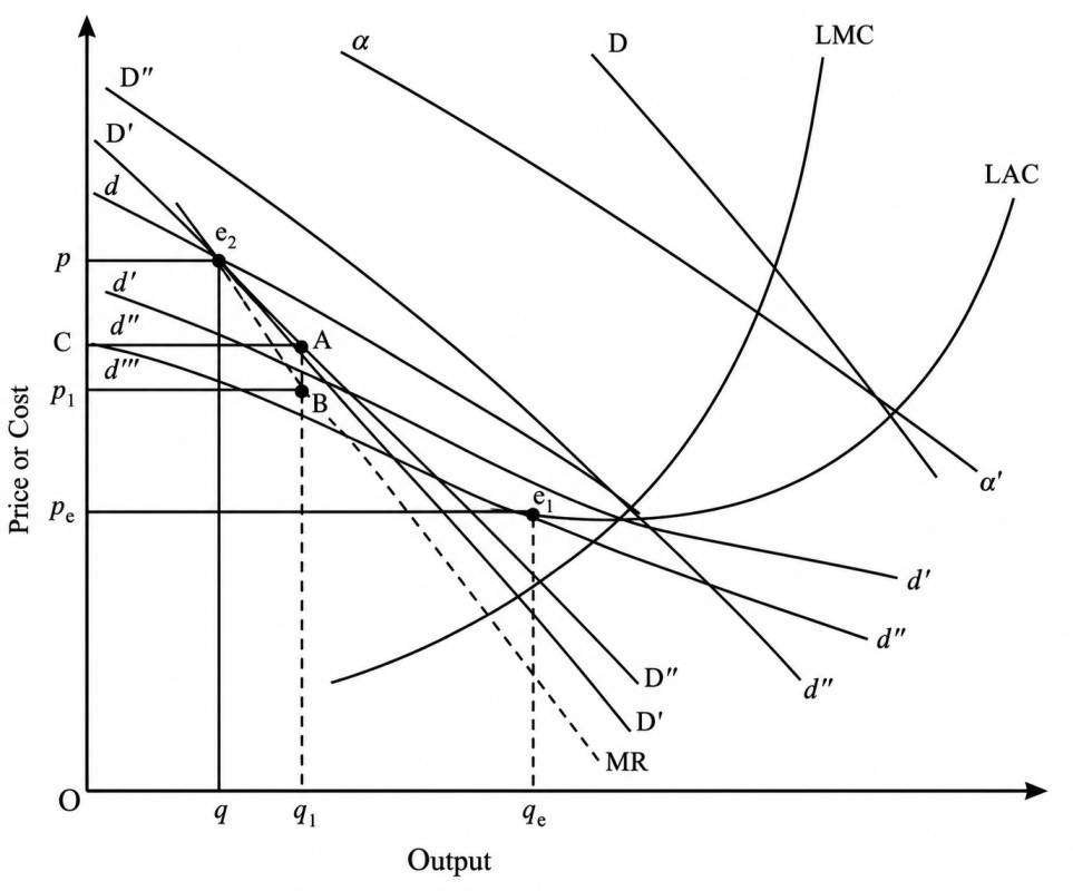
• It is assumed that profits are abnormal at point \(e_1\) as given in Fig. 19. Because of the attraction of abnormal profits, the new firms enter the new product group. As a result of this (DD) shifts to (D’D’). One may think that \(e_2\) is a long-run equilibrium with price (p) and quantity (q) since only normal profits are earned by the firm. Now each entrepreneur’s (dd) is the demand curve and he feels that if he reduces his price his sale would expand along (dd) and profit would increase.

• Each firm is acting in the same way and they also reduce their prices. As price is reduced by all firms, (dd) slides downward along (D’D’) and each firm realizes a loss instead of profit. For example, at a position (d’d’) the firm has reduced its price to \(p_1\) and all the firms act similarly and \(q_1\) is produced with a total loss equal to the area \(ABP_1C\). The reason for the loss is that the average cost is higher than the price.

• The loss increases still further as (dd) slides further down along (D’D’). The financially weakest firm will eventually leave the product group first and the remaining firms will have a larger share. Hence (D’D’) moves to the right as (D”D”) together with (dd). The exit will continue until (dd) becomes tangent to the LAC curve. Hence the changed (D”D”) cuts the downward (d”d”) at the point of tangency \(e_3\) to the LAC curve. Equilibrium is then stable at point \(e_3\) with normal profits earned by all firms producing quantity \(q_e\) at price \(p_e\). The firm will not enter or exit the product group. At this point, the LMC is equal to the MR.

Oligopoly and Duopoly Markets

• An oligopoly market is said to exist when there is a small number of sellers in the market. If two sellers are in the market, the duopoly market exists. The price, quantity, and profit of an oligopolist and duopolist depend upon the action of all producers who are producing identical products. Interdependence of the different actions of the sellers is the main feature of these markets. The profit of each producer is the result of the interaction of the decisions of his rivals.

• There are no generally accepted behavior assumptions for oligopoly and duopoly markets as in the case of perfectly competitive and monopoly markets. Each market solution for a producer is based upon a different set of behavior assumptions. Some of the important solutions are discussed in the following sub-sections. For simplicity, most of the solutions are developed for the duopoly market but some of the solutions may be used for the oligopoly market.

Cournot’s Solution:

• French economist A. Cournot has developed a classical solution for the duopoly market. The firms are assumed to produce a homogenous product. Secondly, the basic behavior assumption of this solution is that each firm or duopolist maximizes his profit on the assumption that the quantity produced by his rival does not change with respect to his own quantity-producing decision. That is, a competitor or rival will not change his output, and he decides his own output so as to maximize profit.

• In this case, the inverse demand function is considered. That is, price is a function of the aggregate quantity produced.

$$p = f(q_1 + q_2)$$

• Where \(q_1\) and \(q_2\) are quantity levels of the duopolists.

• The revenue of each duopolist depends upon his own output level and that of price as aggregate quantity i.e.

$$R_1 = R_1(q_1, q_2)$$

$$R_2 = R_2(q_1, q_2)$$

• The costs are different for different duopolists i.e.

$$C_1 = C_1(q_1)$$

$$C_2 = C_2(q_2)$$

• The first-order condition for profit maximization for both the duopolists is:

$$MR_1 = MC_1$$

$$MR_2 = MC_2$$

• That is the first-order condition for attaining maximum profit requires that each duopolist equates his marginal revenue to its marginal cost. The second-order condition requires that the MR curves cut the MC curves from below.

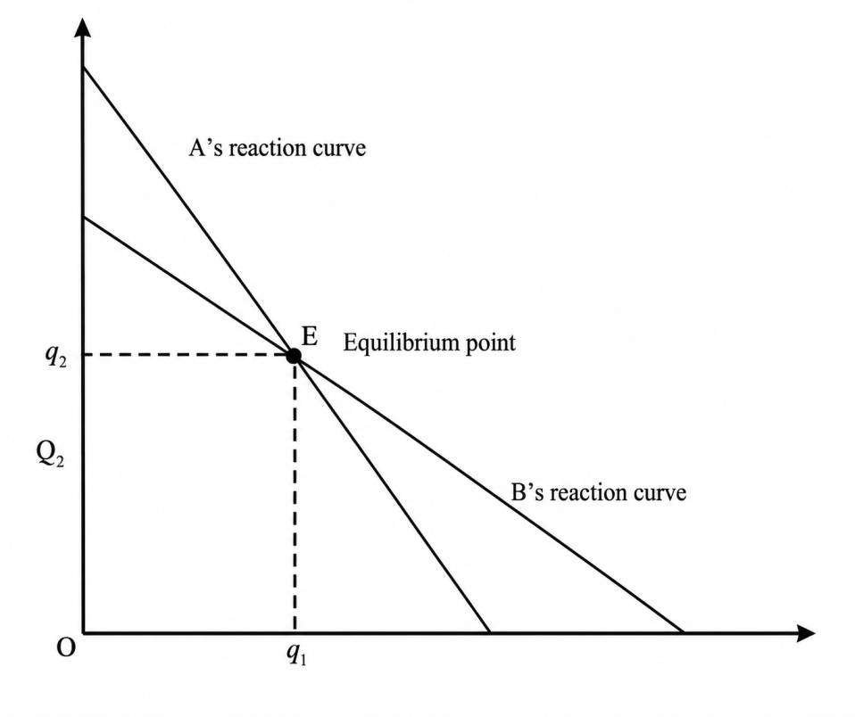
• Solving the first equation for \(q_1\) as a function of \(q_2\) gives the reaction function for the first duopolist. Similarly, the second equation for \(q_2\) in terms of \(q_1\) gives the reaction function for the second duopolist. These equations or reaction functions may be depicted with the graph (Fig. 20). The point of intersection of the two reaction curves will give the equilibrium quantity \(q_1\) and \(q_2\) produced by the first duopolist and second duopolist respectively.

• Mathematically, by solving the first and second equation simultaneously we can get the equilibrium quantity \(q_1\) and \(q_2\) for the first and second duopolist respectively. This is known as the Cournot solution or equilibrium. Equilibrium is reached through a sequence of adjustments of the outputs of duopolists. Cournot’s solution is easily extended to the markets having more than two sellers say oligopoly market.

Collusion Solution:

• Duopolists and oligopolists have mutual interdependence. They produce a homogenous product for selling in the market. Direct agreement among duopolists or oligopolists is an example of collusion. There are several types of collusion namely cartels, market sharing, price leadership, etc. Here we shall discuss the cartels aiming at joint profit maximization of the industry. Here the duopolists or oligopolists are agreed upon the maximization of the total profit of the industry. Both variables i.e. quantity produced and price of product are then under a single control and the industry. It is, in fact, like a monopoly. This situation is identical to that of the multiplant monopolist who produces in two or three plants and maximizes the total profit whereas the costs are different for the product in different plants.

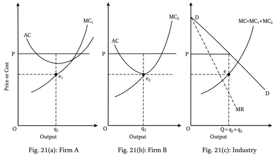
• For simplicity, we assume that there are two firms (duopoly) in the cartel. Their cost structures are different and are given in Fig. 21(a) for A firm and in Fig. 21(b) for firm B. Their marginal costs are \(MC_1\) and \(MC_2\) and the aggregate marginal cost (MC) is the horizontal summation of the individual MCs which is presented in Fig. 21(c). The market demand curve is DD and the marginal revenue of the output of the cartel as a whole is MR.

• The condition for maximization of the total profit of the industry is that the aggregate MC should be equal to the MR of the output as a whole. You will find in Fig. 21(c) that the equilibrium point is at ‘e’ where aggregate MC cuts to MR from below. The equilibrium price is P and the total quantity produced is:

$$(q_1 + q_2)$$

• For individual firms, the first-order condition for profit maximization requires that the marginal cost of each firm must be equal to the marginal revenue of the output as a whole i.e.

$$MC_1 = MC_2 = MR$$

• At this condition, firm A has the equilibrium at ‘\(e_1\)’ and is producing the quantity \(q_1\) and firm B has the equilibrium at ‘\(e_2\)’ and is producing the quantity \(q_2\) at price P.

• Although this solution is very easy to drive but in practice, these cartels rarely have achieved the maximum joint profits due to several reasons such as wrong estimation of the demand curve and marginal cost curve, slow negotiations of cartels, existing high-cost firms, fear of entry of new firms, government interference, etc.

Collusion Solution

Market Sharing Solution:

• In this case, the firms of the industry agree on the share of the total sales of products by an individual firm. That is the share of each firm in the total product has some proportion say equal proportion or one third and two-third. For example, there are two firms (duopoly) in the market and have an equal share in the total product selling in the market. That is the market sale is being shared equally between two firms.

• The firms have identical costs. Each firm will act like a monopolist. The equilibrium of each firm is at the point where the MC of each firm is equal to the MR, and each firm is producing half of the total product at price (p) is determined by the equality of the aggregate MC and MR. The quantity \(q_1\) and \(q_2\) of the product are produced by the Ist and IInd firms respectively. Hence (q) (total product) is:

$$q = q_1 + q_2$$

• If the costs of the firms are different the shares of the market will differ.

Stackelberg’s Solution:

• This solution was developed by the German economist H.V. Stackelberg and it is an extension of Cournot’s model. The firms in the industry are producing homogenous products. In this model one of the firms is a leader and the other firms are the followers. There are two possibilities in which the stable equilibrium emerges:

  • (i) Firm A is the leader and firm B is the follower.

  • (ii) Firm B is the leader and firm A is the follower.

• We shall discuss the case (i) in which firm A is the leader and firm B is the follower as a rival. Firm A determines the reaction function of the follower firm B and substitutes this reaction function with his own profit function. Firm A maximizes its profit like a monopolist and produces a \(q_1\) level of output. Firm B considers the \(q_1\) level of output of firm A and substitutes in its reaction function producing \(q_2\) level of output.

• For example, the aggregate demand function is:

$$p = f(q_1, q_2)$$

• and marginal costs of firm A and firm B are \(MC_1\) and \(MC_2\).

• For profit maximization:

$$MR = MC_1$$

$$MR = MC_2$$

• These conditions are derived from the profit maximization condition of both firms. By solving equations first and second we shall get the reaction equation of firm A in terms of \(q_2\) and the reaction equation of firm B in terms of \(q_1\).

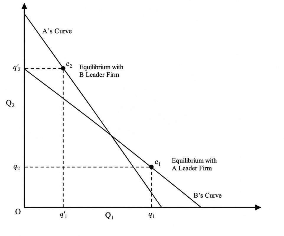
• Now if firm A is the leader, firm A will substitute the reaction equation of firm B in its profit function and it maximizes the profit like a monopolist with the condition of equality between MR and \(MC_1\). Firm A produces the \(q_1\) quantity of output. After that, the follower firm B considers the quantity \(q_1\) of output produced by firm A and substitutes in its reaction equation and produces the \(q_2\) quantity of output. These reaction curves are presented in Fig. 22. The quantity produced by firm A and firm B is \(q_1\) and \(q_2\) respectively.

• Similarly, we can discuss the case (ii) in which firm B is the leader and firm A is the follower. This situation is presented in Fig. 22. The quantity produced by firm B and firm A is obtained as \(q_2’\) and \(q_1’\) respectively.

The Kinked Demand Curve Solution:

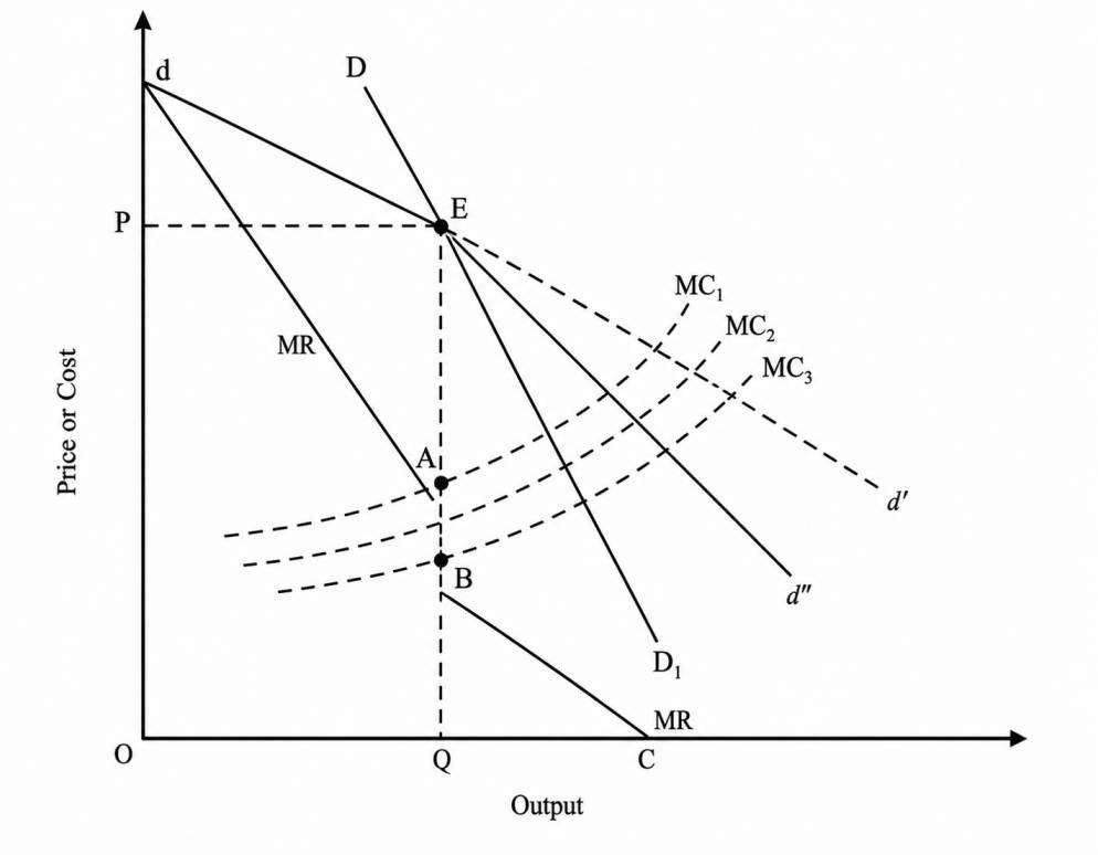
• This solution was given by Paul Sweezy for a stable oligopoly price. In duopoly and oligopoly markets, the prices are frequently changing. Firms in such markets do not change equilibrium prices and quantity due to changes in their costs. The main reason is that if one of the duopolists decreases his price for increasing his sale he expects that his rival will follow suit, matching the price decrease. On the other hand, if one of the duopolists raises his prices, his rival is assumed to change but he does not change his price. Thus the price decrease will be followed by his rival but the price increase will not be followed. This behavioral pattern has a ‘Kink’ in the demand curve (dd’) at point E (Fig. 23) where the price is P. The price reduction below ‘P’ is the relevant demand curve (Ed’) for decision making and for price increase above P is the relevant demand curve (dE). The upper section of the kinked demand curve has higher price elasticity than the lower part.

• Due to the Kink in the demand curve of the duopolist, his MR curve is discontinuous at the level of output corresponding to the kink. The MR has two segments: segment dA corresponds to the upper part of the kinked demand curve while the segment BC corresponds to the lower part of the demand curve. At point E, however, there is finite discontinuity represented by the AB segment of MR.

• The equilibrium of the firm is defined by the point of the kink because at any point to the left of the kink at E, MC is below the MR while to the right of the kink the MC is more than the MR. Thus the total profit is maximized at point ‘E’ of the kink. The equilibrium price is ‘P’ and the quantity is ‘Q’. However, this equilibrium is not necessarily defined by the intersection of the MC and the MR curve. The MC curve passes through anywhere of the discontinuous segment AB of the MR, and the equilibrium price and quantity remain the same. This discontinuity (between A & B) of the MR curve implies that there is a range within which costs may change without affecting the equilibrium P and Q of the firm. According to Sweezy, oligopoly price tends to be very sticky.

• Hall and Hitch use the kinked demand curve in order to explain the ‘stickiness’ of prices in an oligopolistic market but do not use it as a tool for the determination of the price itself.

Efficiency of a Competitive Market

Introduction

• The Central Economic problem revolves around the notion of scarcity which arises when limited resources are rendered to satisfy unlimited wants. The mismatch between needs and means to satisfy those needs exists everywhere. Be it a consumer attempting to maximise his utility constrained by his limited budget, or a producer whose main concern is to maximise profit by minimising costs of production—all aim at attaining maximum gains from the limited resources. This is where originates the concept of Economic Efficiency.

• Efficiency in literal sense refers to the process of outcome generation at lowest possible cost. This in turn results when resources are employed in the best possible way without any wastage. In Economics, Pareto optimality and efficiency are often used synonymously. An allocation is referred to as being Pareto optimal/efficient when there exist no alternate allocations which can make someone better off without making someone else worse off.

• The present unit begins with explaining the concept of Efficiency in a General Equilibrium framework. Subsequently, necessary tools of this framework encompassing the Edgeworth box, Pareto optimal allocation, and market trade leading to achievement of a Competitive Equilibrium, are discussed to explain the mechanism and the outcome of a free market. This theoretical stage is then followed by the algebra of General equilibrium, and later by the Walras’ law.

• The two bases, one—the concept of Pareto optimality or efficiency and the other—the mechanism of reaching a competitive equilibrium by a free market, will then be combined to establish the notion of “efficiency of a competitive market”—this will then be underlined by the First Fundamental theorem of Welfare Economics. The first fundamental theorem of welfare simply claims—a competitive equilibrium is Pareto efficient. This is equivalent to say, competitive equilibrium results in efficient resource allocation, so that no alternate allocation could enhance gain to someone without harming someone else.

• Possibility of social undesirability of Pareto optimal allocation also exists. This happens when the justice and fairness in terms of distribution of efficient allocation of resources are brought into consideration. The Second fundamental theorem of Welfare Economics then comes into picture. Under certain assumptions, it separates the goals of Efficiency and Equity, emphasising that a society may achieve any Pareto optimal resource allocation through appropriate initial resources redistribution and free trade.

The Concept of Efficiency

• Scarcity of resources is the fundamental economic problem. As a rescue to this problem, Efficiency is concerned with optimal allocation of resources among different economic agents. In absolute terms, a situation can be called economically efficient if and only if— no one can be made better off without making someone else worse off. This is referred to as the Pareto efficient/optimal condition. An efficient condition could also be said to result when it becomes impossible to generate additional output unless amounts of factors employed are increased. In other words, it will not be wrong to say that in an efficient situation, production proceeds at the lowest possible per-unit cost. These statements claiming efficiency are not exactly equivalent, but they all dictate the idea that a system is said to be efficient if nothing more can be achieved given the available resources.

• The equilibrium concepts you have used till now in the earlier units, are what is referred to as attainment of equilibrium by way of partial equilibrium analysis. As the name suggests, such equilibrium is achieved in one market holding what occurs in other markets, constant. This assumption would be correct when a market operates in isolation. A scenario of isolation does not exist in the present world. There exist complex interconnections between each market and firm. To get a broad view of the efficiency criterion in case of a competitive market, we will look into the general equilibrium framework. The criteria of efficiency will be discussed, based on which efficiency of a competitive market will be touched upon.

• To set the stage for explaining the concept of efficiency in a general equilibrium framework, we will be adopting the following three essential assumptions that will simplify our analysis. Nonetheless, the results are still applicable in a general case.

  • Consumers and producers operate in competitive markets, implying all agents are price takers, and achieve equilibrium, given the prices.

  • There are only two goods which are produced using only two factors of production.

  • There are two consumers, each endowed with a certain quantities of the two goods which they will trade among themselves.

• Initially, we will ignore production and will just consider attainment of equilibrium in consumption case. We will assume that the two consumers are each endowed with a certain quantities of the two goods, and then we will examine how they achieve equilibrium through trade with one another. This is what is typically termed a Pure Exchange economy. The approach adopted will be further extended to the efficiency attainment in production case and then to efficient allocation of two goods produced.

Pareto Optimality

• Named after the economist Vilfredo Pareto, Pareto Optimality refers to an economic arrangement where resources are allocated in such a way that there exist no alternative feasible resource allocation which will make one person better off without making someone else worse off.

• In this context, given a set of alternative allocations of resources, if a change from one allocation to another can make at least one individual better off without making any other individual worse off, it is referred to as Pareto improvement.

• Consequently, an allocation will be Pareto optimal when no further Pareto improvements can be made.

Edgeworth Box and Pareto Optimal/Efficient Allocations:

• Edgeworth box is a powerful graphical tool in General equilibrium analysis to study the goods trade in the market for attaining efficiency. In order to bring two agents in the market under one roof, it merges their indifference maps by inverting one of the agents ICs. The box depicts all possible consumption bundles for both consumers under examination (i.e. all feasible allocations), as well as preferences of both the individuals.

• Consider a hypothetical market situation with two consumers in the economy, A and B and consuming two goods, x and y. Let A’s consumption bundle be given by:

$$X_A = (x_A, y_A)$$

• Where:

$$x_A$$

denotes A’s consumption of good x and \(y_A\)

of good y. Similarly,

$$X_B = (x_B, y_B)$$

represents consumption bundle of consumer B.

• Furthermore, let:

$$\omega_A = (\omega_x^A, \omega_y^A)$$

denote an initial endowment bundle of consumer A and \(\omega_B = (\omega_x^B, \omega_y^B)\)

of consumer B.

• Now assume:

$$\omega_A = (4, 1)$$

$$\omega_B = (4, 5)$$

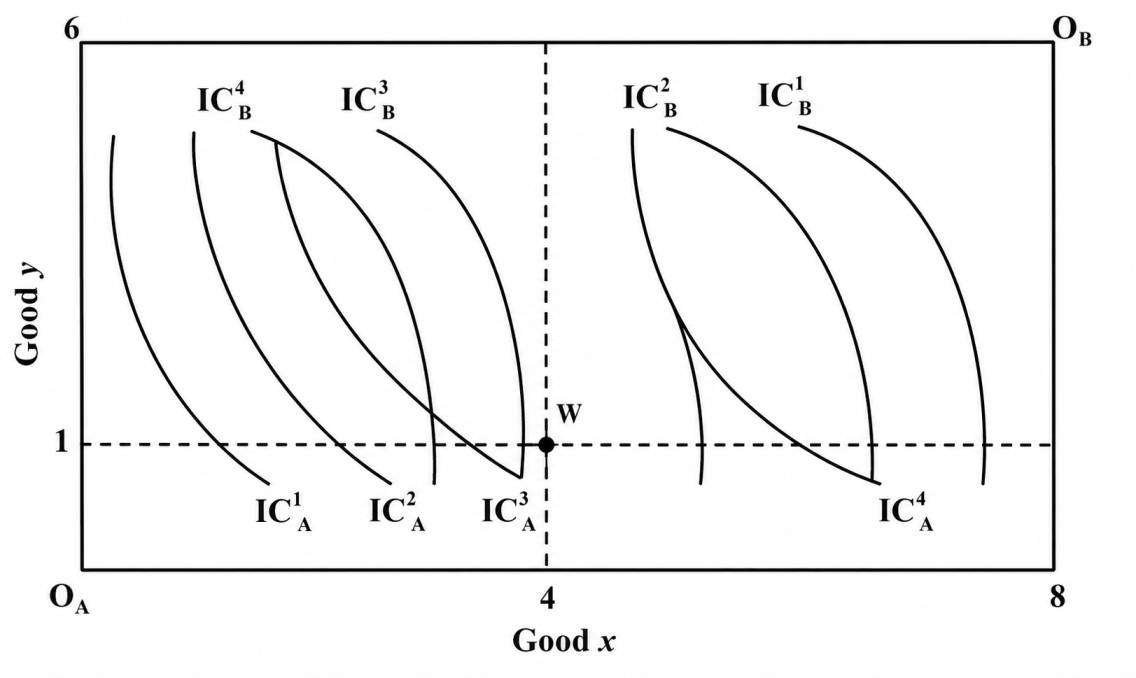
An Edgeworth box is given in Fig. 24. Height of the box measures the total amount of good y in the economy (here, 6 units) and the width measures the total amount of good x (here, 8 units).

• Person A’s consumption choices are measured from the lower left-hand corner (OA), and that of person B’s from the upper right-hand corner (OB). Recall that any point inside the Edgeworth box indicates a particular distribution of the two goods among the two individuals. ‘W’ represents the initial endowment allocation. ICA and ICB are the Indifference curves representing preferences of consumer A and B, respectively.

Important:

• A pair of consumption bundles (X_A) and (X_B) is an Allocation.

• An allocation is feasible (i.e. affordable), if and only if,

$$x_A + x_B = \omega_x^A + \omega_x^B$$

$$y_A + y_B = \omega_y^A + \omega_y^B$$

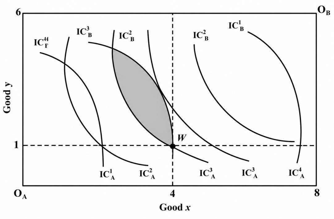
• Now consider Fig. 25, notice that ICs of both individuals pass through W (i.e. the endowment). This implies that agents A and B are indifferent to their endowment allocation W compared to another points along the ICs passing through it. Further, note that all the consumption bundles to the north-east of the indifference curve that passes through W yield a higher level of utility for agent A.

• Similarly, all points to the south-west of the inverted indifference curve passing through W are preferred by agent B. The lens-shaped area (the shaded region) formed by ICs of both the individual passing through W represents a set of allocation bundles that would make both consumer A and B better off compared to their initial endowment.

• This is what we referred to as the Pareto Improvement. Possibility of Pareto improvement in turn suggests that there can be a possibility of an equilibrium allocation, but will that be a unique one?

• Suppose scope of Pareto improvement seizes at point Q (refer Fig. 26). It is easy to see that consumer A could achieve it by trading her endowment of good x to consumer B in return for her endowment of good y. Such a trade will allow agent A to reach a higher level of utility by consuming more units of good y than he was endowed with. Similarly, consumer B would enjoy higher utility by consuming more of good x than the amount he was endowed with.

• No reallocation from point Q can make one consumer better off without making the other worse off. An allocation of such kind is called Pareto efficient/optimal allocation, given the initial endowment bundle W and preferences of both the consumers. At such an allocation, all gains from trade are exhausted.

• Notice that at Pareto efficient allocation Q, Marginal Rate of Substitution (MRS) is same for both the consumers. This is represented by the tangency of their respective ICs at Q. This tangency is necessary otherwise it will still be possible for them to trade to another level within the lens-shaped area.

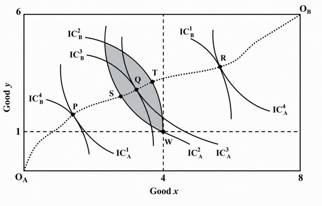
• Remember that, Pareto efficient point (Q) is not unique. We attained such an allocation for the given initial endowment W. With change in the endowment, there will be a resultant change in the optimal bundle. Thus, there exists infinite number of efficient points— the set of which is called a Pareto Set or the Contract Curve (dotted line in Fig. 26).

• A Pareto Set is composed of all the possible allocations resulting from mutually advantageous trade from any given endowment. This curve will stretch from A’s origin to that of B’s. It is a locus of all the points where ICs of the agents will be tangent. Points P, Q, and R, represent three such points.

• Please note: For a given endowment (here W), there exists a subset of Pareto set (here, curve ST) inside the lens-shaped region formed by ICs passing through that endowment.

Market Trade for Equilibrium Attainment:

• Now, let us discuss the mechanism to be adopted in order to reach an optimal/efficient allocation (like Q) on the contract curve. Recall the procedure involved for attaining equilibrium by a consumer that we learnt in Unit 2. An individual attains equilibrium when his indifference curve is tangent to his budget constraint.

• That is, when slope of IC (which is MRS) = Price ratio \(\left(\frac{P_x}{P_y}\right)\), slope of budget constraint [which is the Price ratio with \(P_x\) and \(P_y\) being prices of good x and good y, respectively].

\[ MRS=\frac{P_x}{P_y} \]

• We have just learnt— a contract curve is nothing but a locus of all equilibrium allocations so that MRS between two goods (say x and y) is equal among two consumers (say A and B). This equality does not happen at all price ratios, but only at the one where the market clears, i.e. at price ratio so that:

\[ MRS_A=MRS_B=\left(\frac{P_x}{P_y}\right)^* \]

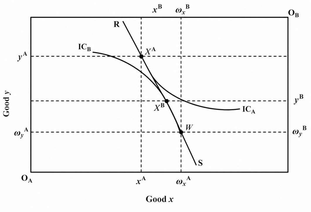
• Consider a market situation represented by an Edgeworth box in the Fig. 27. Given the two individuals (A and B), participating in the consumption of two goods (x and y), in order to maximise the utility, represented by their ICs \((IC_A)\) and \(IC_B\), for individual A and B, respectively). Let the initial endowment be represented by bundle:

\[ W=\left((\omega_x^A,\omega_y^A),(\omega_x^B,\omega_y^B)\right) \]

• Budget line RS represents a price ratio at which both the individual decides to trade with each other. At this price ratio, individual A demands bundle:

\[ X^A=(x^A,y^A) \]

and individual B demands bundle:

\[ X^B=(x^B,y^B) \]

• As you may notice, Demand for Good 1 is feasible, only when Demand for Good 2 is feasible.

\[ x^A+x^B=\omega_x^A+\omega_x^B \]

\[ y^A+y^B=\omega_y^A+\omega_y^B \]

• In other words, feasibility condition requires, excess demand of individual A (or B) for good (i) (where:

\[ i\in\{x,y\} \]

must match excess supply of individual B (or A) for that good.

• But in Fig. 27, this is not the case, as excess supply of good x by individual A, denoted by:

\[ ex^A=(\omega_x^A-x^A) \]

is greater than excess demand for good x by individual B, given by:

\[ ex^B=(x^B-\omega_x^B) \]

Similar situation exists for good y. Hence, the above situation depicts a situation of Disequilibrium in the exchange market.

• Symbolically,

\[ x^A+x^B\neq\omega_x^A+\omega_x^B \]

\[ y^A+y^B\neq\omega_y^A+\omega_y^B \]

Competitive Equilibrium

• In Fig. 27, there is disequilibrium in the market due to presence of excess demand for good y and excess supply for good x. The prices in the above market need to be recalibrated to the point where aggregate demand for a good equals its aggregate supply, i.e. when amount of a good demanded by one individual is exactly equal to the amount supplied by the other. Only then, the market is in a Competitive Equilibrium. This equilibrium is also called Walrasian Equilibrium.

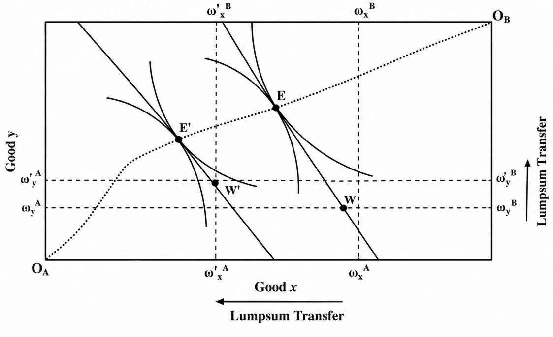
• In Edgeworth box setting, a competitive equilibrium results when ICs of both the individuals become tangent to each other at the ongoing price ratio. This happens on the contract curve, at the price ratio which equilibrate the trade for utility maximisation, given the initial endowment. One such equilibrium is given by point E in Fig. 28, where the budget line through the endowment point passes through the tangency of the ICs of the two individuals A and B.

• Point E ensures that both individuals attain maximum utility by reaching their highest possible IC through trade, given their initial endowment bundle W. Trade leading to equilibrium outcome happens at a unique price ratio given by the slope of the budget line passing through common tangency point and the initial endowment bundle W.

\[ \left(\frac{P_x}{P_y}\right)^* \]

• Thus at equilibrium, the following must be true:

\[ MRS_A=MRS_B=\frac{P_x}{P_y} \]

or

\[ \frac{MU_x^A}{MU_y^A}=\frac{MU_x^B}{MU_y^B}=\frac{P_x}{P_y} \]

• Note: A price ratio and an allocation given by:

\[ [(x^A,y^A),(x^B,y^B)] \]

is a competitive equilibrium if the following condition holds:

• Each consumer is maximising his/her utility given his/her budget set.

• The demand for and the supply of each good are equal, i.e. markets clear.

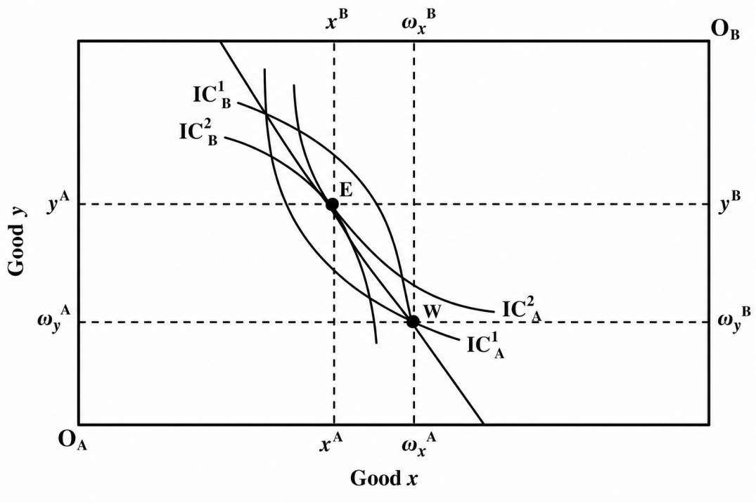
General Equilibrium and Walras’ Law

Algebra of General Equilibrium:

• Market economies are composed of a complex dynamic system of different economic agents, making supply and demand decisions over different commodities or factor types in order to maximise their own interests. General Equilibrium theory advocates that such pursuit of private interest by all the economic units with different motivations, integrated through a system of free markets, will result in an efficient/optimal allocation of goods and services in the economy.

• By General equilibrium it is meant simultaneous equilibrium in all the markets, that is, the prevalence of equilibrium in the economy as a whole. A General Equilibrium results in an array of prices for all goods so that supply equals demand simultaneously for each good in the economy. We establish the algebra of such equilibrium below.

• Assuming two commodities (x and y) and two agents (A and B) in the economy, then a typical array of prices is given by a two-dimensional vector such as:

\[ (P_x,P_y) \]

Let the demand function for agent A be:

\[ x^A(P_x,P_y) \]

and

\[ y^A(P_x,P_y) \]

for commodity x and commodity y, respectively. Similarly for agent B will be given by:

\[ x^B(P_x,P_y) \]

and

\[ y^B(P_x,P_y) \]

Further their endowment bundle be:

\[ (\omega_x^i,\omega_y^i), \quad i\in\{A,B\} \]

• General Equilibrium in the economy would be established by a price vector:

\[ (P_x,P_y) \]

so that Aggregate Demand = Aggregate Supply, for each commodity. That is,

\[ x^A(P_x,P_y)+x^B(P_x,P_y)=\omega_x^A+\omega_x^B \]

\[ y^A(P_x,P_y)+y^B(P_x,P_y)=\omega_y^A+\omega_y^B \]

• The above equation can be arranged in terms of Excess demand functions for the two agents:

\[ [x^A(P_x,P_y)-\omega_x^A]+[x^B(P_x,P_y)-\omega_x^B]=0 \]

\[ [y^A(P_x,P_y)-\omega_y^A]+[y^B(P_x,P_y)-\omega_y^B]=0 \]

• Where,

\[ [x^A(P_x,P_y)-\omega_x^A] \]

is the excess demand for commodity x by agent A, similarly,

\[ [x^B(P_x,P_y)-\omega_x^B] \]

is the excess demand for commodity x by agent B. Equation (10) simply says, equilibrium calls for the sum of the excess demands for commodity x by both the agents to sum to zero. In other words, at equilibrium, one agent’s demand for a good must equal another agent’s supply of that good. This is another way of looking at the condition of feasibility of the demand for a commodity. Equation (11) can be interpreted in a similar way.

• Above equations can also be presented as follows:

\[ e_x^A(P_x,P_y)+e_x^B(P_x,P_y)=0 \]

Where,

\[ e_x^A(P_x,P_y)=[x^A(P_x,P_y)-\omega_x^A] \]

and

\[ e_x^B(P_x,P_y)=[x^B(P_x,P_y)-\omega_x^B] \]

Similarly, for commodity y, Equation becomes:

\[ e_y^A(P_x,P_y)+e_y^B(P_x,P_y)=0 \]

• Further let,

\[ e_x^A(P_x,P_y)+e_x^B(P_x,P_y)=z_x(P_x,P_y) \]

and

\[ e_y^A(P_x,P_y)+e_y^B(P_x,P_y)=z_y(P_x,P_y) \]

then General Equilibrium condition can be stated more precisely as:

\[ z_n(P_x,P_y)=0,\quad \text{where } n\in\{x,y\} \]

Walras’ Law:

• Walras’ Law is given by:

$$P_xZ_x(P_x,P_y)+P_yZ_y(P_x,P_y)=0$$

• The law simply says that for all prices (and not just the equilibrium prices) the value of aggregate excess demand is identically zero. The proof of the law is as follows.

• Feasibility of demand by agent A requires:

$$P_xx^A(P_x,P_y)+P_yy^A(P_x,P_y)=P_x\omega_x^A+P_y\omega_y^A$$

$$P_x[x^A(P_x,P_y)-\omega_x^A]+P_y[y^A(P_x,P_y)-\omega_y^A]=0$$

$$P_xe_x^A(P_x,P_y)+P_ye_y^A(P_x,P_y)=0$$

• Similar equation holds for feasibility of demand by agent B:

$$P_xe_x^B(P_x,P_y)+P_ye_y^B(P_x,P_y)=0$$

• Adding Equations (12) and (13), we get:

$$P_xe_x^A(P_x,P_y)+P_ye_y^A(P_x,P_y)+P_xe_x^B(P_x,P_y)+P_ye_y^B(P_x,P_y)=0$$

$$P_x[e_x^A(P_x,P_y)+e_x^B(P_x,P_y)]+P_y[e_y^A(P_x,P_y)+e_y^B(P_x,P_y)]=0$$

$$P_xZ_x(P_x,P_y)+P_yZ_y(P_x,P_y)=0$$

• Significance of the Walras’ law— Given that a set of prices bring equilibrium in any one of the markets (let say in market for good x), then as per Walras’ law the remaining markets (here market for good y) would be necessarily in equilibrium. In other words, the law claims that if demand equals supply in one market then the same must be true for the other market as well.

• From the identity of the law:

$$P_xZ_x(P_x,P_y)+P_yZ_y(P_x,P_y)=0$$

if

$$Z_x(P_x,P_y)=0$$

that is, if market for good x is in equilibrium so that supply equals demand for good x. Given that both \( P_x \)  and \( P_y \)  are positive, for the identity of Walras’ law to hold true, then \( Z_y(P_x,P_y)=0 \)

must also equal 0.

• It turns out that if demand equals supply in all but one market, i.e. in \((n-1)\) markets, then demand must equal supply in the \(n^{th}\) market as well. This has an added advantage to it, for an economy with (n) goods, one of the prices can be chosen as numeraire price (a price relative to which all the other prices are measured), leaving the need to find only \((n-1)\) relative equilibrium prices.

• This becomes possible from the Walras’ law identity that states all markets would be in equilibrium for any set of prices. This is to say, if markets are in equilibrium at a price vector:

$$(P_1,P_2,P_3,\ldots,P_n)$$

then for any constant

$$k\in\mathbb{R}^{+}$$

(set of positive real numbers), markets will remain in equilibrium for a price vector:

$$(kP_1,kP_2,kP_3,\ldots,kP_n)$$

• Now, if we take:

$$k=\frac{1}{P_n}$$

then \( P_n \)  becomes the numeraire price which will then result in a price vector of \((n-1)\) relative equilibrium prices, given by: \( \left(\frac{P_1}{P_n},\frac{P_2}{P_n},\frac{P_3}{P_n},\ldots,1\right) \)

The Efficiency of Competitive Equilibrium

• On combining Pareto Optimality and Competitive Equilibrium (Section 8.4) conditions, efficiency of a competitive equilibrium can be verified. In a competitive equilibrium, the amount supplied of a good equals the amount demanded. This eliminates the scope for further gains from trade or any reallocation— which is nothing but the condition that needs to hold for an efficient allocation.

• Competitive equilibrium E in Fig. 28 is efficient with each individual A and B reaching the highest possible IC given their initial endowment W, so that neither A nor B can be made better off without making the other individual worse off. A general proof verifying efficiency of a competitive equilibrium is as follows.

• Consider the similar situation that we have been considering so far, of two goods (x and y) and two individuals (A and B), with initial endowment:

$$W=[(\omega_x^A,\omega_y^A),(\omega_x^B,\omega_y^B)]$$

Further let trade at price ratio:

$$p=\left(\frac{P_x}{P_y}\right)$$

lead to competitive equilibrium bundle:

$$E=[(x^A,y^A),(x^B,y^B)]$$

• Now, suppose equilibrium bundle E is not Pareto efficient. This would mean that there exists an alternate allocation which will be strictly preferred by A and B to:

$$(x^A,y^A)$$

and

$$(x^B,y^B)$$

respectively. Let it be given by:

$$[(x_a^A,y_a^A),(x_a^B,y_a^B)]$$

That is,

• For individual A, \( (x_a^A,y_a^A)>(x^A,y^A) \)

• For individual B, \( (x_a^B,y_a^B)>(x^B,y^B) \)

• The preferred allocation must be feasible, that is,

$$x_a^A+x_a^B=\omega_x^A+\omega_x^B$$

$$y_a^A+y_a^B=\omega_y^A+\omega_y^B$$

• Now, since individual A prefers: \( (x_a^A,y_a^A) \) to \( (x^A,y^A) \) and given that at price ratio: \( p=\left(\frac{P_x}{P_y}\right) \) he opted for: \( (x^A,y^A) \) then at (p), bundle: \( (x_a^A,y_a^A) \) must be unaffordable for A. This implies: \( P_xx_a^A+P_yy_a^A>P_x\omega_x^A+P_y\omega_y^A \)

• The above equation simply means that the money value of bundle: \( (x_a^A,y_a^A) \) at the given price ratio exceeds the money value of bundle: \( (x^A,y^A) \) opted by A at that price ratio.

• Similarly for individual B the following relation will hold: \( P_xx_a^B+P_yy_a^B>P_x\omega_x^B+P_y\omega_y^B \)

• Adding (15) and (16), we get:

$$P_xx_a^A+P_yy_a^A+P_xx_a^B+P_yy_a^B>P_x\omega_x^A+P_y\omega_y^A+P_x\omega_x^B+P_y\omega_y^B$$

$$P_x(x_a^A+x_a^B)+P_y(y_a^A+y_a^B)>P_x(\omega_x^A+\omega_x^B)+P_y(\omega_y^A+\omega_y^B)$$

The First Fundamental Theorem of Welfare Economics:

• As per the First Fundamental Theorem of Welfare Economics, all competitive equilibria or Walrasian equilibria are Pareto Efficient. The theorem claims that a competitive equilibrium will exhaust all gains from trade so that an efficient allocation is attained from any given initial endowment. This theorem confirms to the result of the classical theory, viz. the Adam Smith’s “invisible hand” hypothesis, as per which invisible hand of the market forces of demand and supply will achieve most efficient level of production, consumption and distribution of good in the society.

• First Fundamental Theorem of Welfare Economics supports the case for “free markets” or “Laissez-faire”, where there exists no control by the government on production or consumption that may interfere with the free market. Only when the market mechanism fails to achieve an efficient resource allocation (which is the case of market failure resulting from monopoly, externalities, or public goods), the government intervention is justified.

• However, the First Fundamental Theorem— which talks about the Pareto efficiency of a competitive equilibrium— says nothing about equity or fairness of the resulting efficient resource allocation among the agents of a society. Pareto efficiency merely indicates that no one can be made better off without making someone else worse off, it gives no consideration to the distributive effects of the resultant efficient allocation.

• The point to note here is— Laissez-faire may produce many different Pareto optimal outcomes, with some being fairer than others, so that not all of them may be equally desirable by the society. For instance, the outcome in which one individual A has all the units of commodity x in a single commodity market is Pareto efficient, since there will be no way to make some other individual better off without making A worse off. But such an optimal allocation may not be equitable or socially desirable.

• This is where the need for rectifying the distributional inequities of Laissez-faire comes. Now we proceed towards a socially desirable Pareto optimum solution, with an approach which is converse to that of the First Fundamental Theorem of Welfare Economics, i.e., we are considering the allocation problem from efficiency to equilibrium. Given Pareto Efficient equilibrium, as long as individual preferences are convex, there exists a set of prices at which this equilibrium becomes competitive or Walrasian equilibrium. This is known as the Second Fundamental Theorem of Welfare Economics which we further explain below.

The Second Fundamental Theorem of Welfare Economics:

• The Second Fundamental Theorem of Welfare Economics suggests that the issues of efficiency and equity are distinct, and that they can be addressed simultaneously. As per this theorem, any socially desirable optimal allocation can be reached by way of the market mechanism modified with the help of lump-sum transfers.

• Assuming all agents (individuals and producers) are self-interested price takers, then as per the Second Fundamental Theorem of Welfare Economics, almost any Pareto optimal equilibrium can be achieved through the competitive mechanism, provided appropriate lump-sum transfers (which do not change the agents’ behaviour) are made among agents.

• Consider Fig. 29 below, where we have two Pareto efficient allocations E and Eʹ. If it is felt that equilibrium Eʹ is somehow better in terms of being more fair or just than equilibrium E, then a lump-sum transfer of good X from individual A to B and simultaneously a transfer of good Y from B to A, changing the endowment from W to Wʹ, can be made.

• The price system can then be allowed to generate a Pareto efficient outcome Eʹ, given the new endowment Wʹ. Thus, as per the Second Fundamental Theorem of Welfare Economics— given all agents have convex preferences, after an appropriate assignment of endowments through redistribution, a society may achieve any Pareto efficient resource allocation as competitive equilibrium, that is, through the market mechanism.