Open Economy Models: Mundell and Fleming Model (IS, LM and BP Curve), Balance of Payments, Exchange Rate Determination, Purchasing Power Parity | CUET PG Economics – Notes

Mundell-Fleming Model

Introduction

• The most striking feature of today’s economies is high degree of integration among financial and capital markets. Policymakers have to consider the international exchange rate and interest rate movements while formulating the domestic fiscal and monetary policies. As restrictions on free movement of capital are being dismantled, capital moves to the country which offers highest risk adjusted yield. An expansionary monetary policy reduces the yield of assets by increasing their prices. If this yield falls below the international rate of interest, the international investors will withdraw their money and invest it in other countries where they get higher returns. Capital mobility has thus linked the assets markets of the world together.

• In this Unit we will introduce international trade and finance through the Mundell-Fleming model. We begin by introducing the model for a small open economy in the short run. Subsequently, we introduce the IS-LM-BP framework to study the effectiveness of policies in a small open economy. Thereafter, the effectiveness of monetary and fiscal policies for a country that operates with a floating exchange rate regime (i.e. the exchange rate adjusts freely to changes in economic conditions) is discussed. We conclude by discussing the pros and cons of fixed and floating exchange rate regimes.

The Model

• Before we start with the formal exposition of the Mundell Fleming Model, we must first understand how equilibrium in ‘investment’ (I) is determined for a small open economy. In an open economy, exports (X) just like investment, are an injection into the country’s income stream. They are taken to be autonomous or independent of domestic income. On the other hand, ‘imports’ (M), just like saving (S), represent a leakage out of the income stream. In a small open economy, therefore, the equilibrium condition for investment in the income stream is determined by:
  𝑰 + 𝑿 = 𝑺 + 𝑴 … (1)
  𝑿 − 𝑴 = 𝑺 − 𝑰 … (2)
  The expression (X − M) i.e. ‘net exports’ in equation (2) is equal to net foreign investment. If imports exceed exports, the term (X −M) is negative so that domestic investment exceeds domestic saving by the amount of net foreign disinvestment (i.e., the amount by which foreigners are investing in the country). Developed by Robert Mundell and Marcus Fleming in the 1960s, the Mundell-Fleming model studies the implications of capital mobility under a fixed or flexible exchange rate regime in a small open economy. It is an open economy version of the IS-LM model. It makes one important and extreme assumption, i.e., the economy being studied is a small open economy with perfect capital mobility. This means, the economy can borrow or lend as much as it wants in world’s financial markets and, as a result, the economy’s interest rate is determined by the world interest rate. More specifically, the assumption can be delineated in terms of its three specific respects as follows:

  1. Perfect capital mobility implies that investors can purchase assets in any country they choose, quickly, with low transaction costs and in unlimited amount. With such perfect capital mobility, investors can move capital to the country offering highest return without any restriction. Any change in the rate of interest of any country in the world, will cause capital flows to restore yields to the world level.

  2. Small open economy implies that the interest rate in this economy i, is determined by the world interest rate i* i.e. i= i*. The world interest rate is assumed to be exogenously fixed since the economy, relative to the world economy, can borrow or lend as much as it wants in world financial markets without affecting the world interest rate. This means, not only the rate of interest of a small open economy is determined at the world interest rate, i*, but its ‘balance of payments’ (BoP) are also in equilibrium at i = i*. Thus, an increase in the domestic interest rate ‘i’ above the world rate of interest ‘i*’, will lead to capital inflows into the domestic economy. These inflows will continue till the domestic rate of interest gets aligned with international rate of interest. Similarly, a fall in i below i*, will trigger huge capital outflows. Such capital outflows from the domestic economy will continue till i rises and equals i*. Hence, the i = i* equation represents the assumption that the international flow of capital is rapid enough to keep the domestic interest rate equal to the world interest.

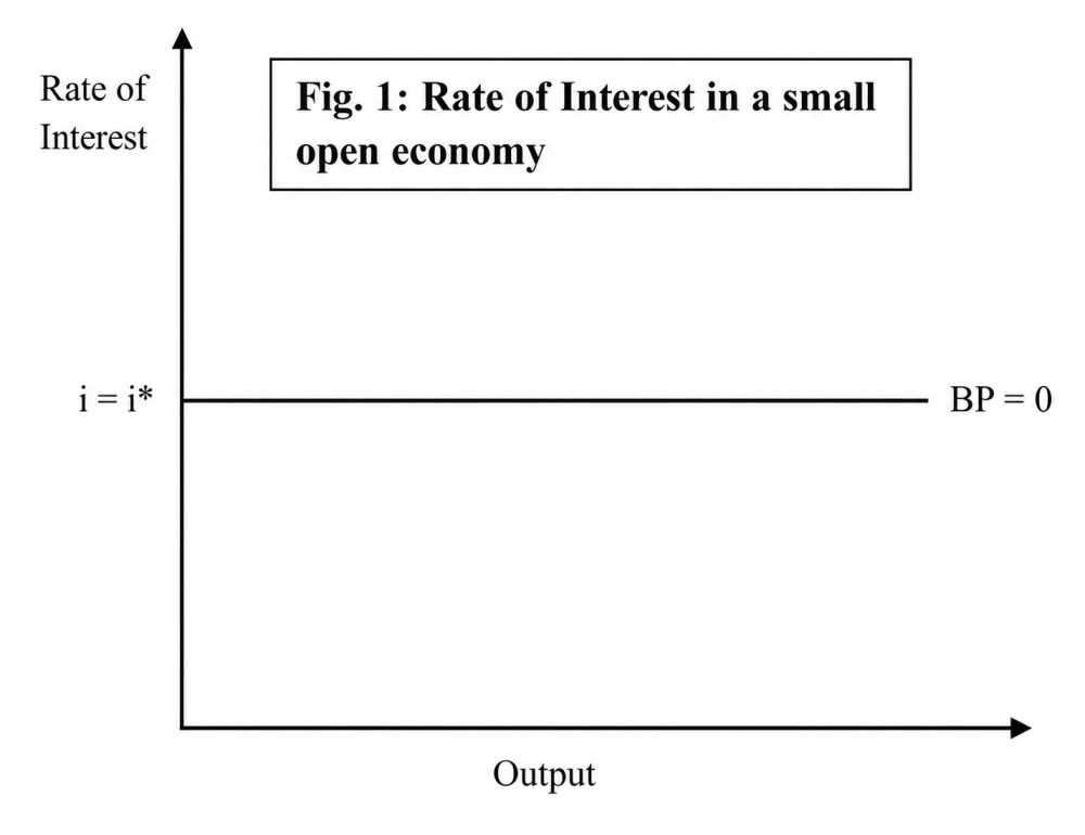
• It is also assumed that the price level at home (P) and abroad (P)* do not vary much i.e. the model is designed for analysing short-run fluctuations. Thus, if ‘e’ is the nominal exchange rate (defined as the amount of domestic currency per unit of foreign currency), a decrease in nominal exchange rate (i.e. appreciation making foreign goods cheaper relative to domestic goods) will cause a proportionate decrease in real exchange rate by ‘e’ equal to: eP/p*.