Permanent, Relative and Life Cycle Hypothesis, Determinants of Business Fixed Investment; Residential Investment and Inventory Investment, Multiplier and Accelerator | CUET PG Economics

The Permanent Income Hypothesis

• Milton Friedman’s famous study entitled A Theory of the Consumption Function published in 1957, also tried to reconcile the short run non proportional income consumption relationship with the long run proportional income consumption relationship. Friedman distinguishes between the current or observed or measured income of any given time period and the permanent income on which the consumers’ base their behavior. Similarly he has distinguished between the current or observed or measured consumption and permanent consumption.

• According to Freidman, permanent income is “the amount a consumer unit could consume (or believes that it could) while maintaining its wealth intact” while permanent consumption is “the value of the services that it is planned to consume during the period in question”. It is the mean income which the family unit regards as permanent and would depend upon the family unit‟s time horizon and farsightedness.

• The permanent income hypothesis states that the ratio of the permanent consumption to permanent income is constant. Since permanent consumption is proportional to permanent income, the long run aggregate APC equals to long run aggregate MPC. Rich and the poor devote the same fraction of their incomes to consumption. In other words, the APC of the families at all levels of their income is constant.

• According to Milton Friedman, observed or measured income and observed and measured consumption of any short period for the economy or the individual is composed of permanent and transitory components. While the permanent components of the measured consumption and measured income are perfectly correlated, the transitory components of the measured consumption and measured income are neither correlated to their corresponding permanent components nor are they correlated to each other.

• The permanent income hypothesis can be explained in the form of following equations-

  • Cp-K(i,w,µ)Yp .(i)

  • b(.YpYt)=0……(ii)

  • Y= Yp+Yt C=Cp+Ct b(Cp Ct)=…(iii)

  • b(Y+ Ct)………….(iv)

• Where

  • Y = measured or observed disposable personal income

  • C = measured or observed consumption

  • Yp = permanent income

  • Y₁= transitory income

  • Cp = permanent consumption

  • Ct = transitory consumption

  • K = proportionality constant between permanent consumption and permanent income

  • i = rate of interest

  • w = ratio of non-human wealth to permanent income

  • μ = propensity of the consumer unit to add to consumption rather than to wealth. Number and ages of the family members, transitory factors affecting income and consumption determine the value of μ.

  • b = coefficient term

• The equation (i) states the relationship between permanent income and permanent consumption. This indicates that long run APC as a ratio of permanent consumption to permanent income is constant, i.e. Cp/Yp = K = constant. K is independent of the level of income. However it gets influenced by the term i, w and μ.

• Equation (ii) states that observed income is composed of permanent income and transitory income.

• Equation (iii) states that the observed or measured consumption is composed of permanent consumption and transitory consumption. Permanent and transitory components are not correlated. Transitory income can be positive or negative, thus making the observed income to be greater or less than the permanent income respectively.

• If a family wage earner receives an extra unexpected special bonus or overtime allowance during the year which he does not expect to receive in the following years, this is a positive transitory component of the current or measured income. In this case, measured income rises above the permanent income.

• On the other hand, if due to a sudden unexpected shut down of the plant the wage earner suffers a loss in his measured income during the year but does not expect to have this loss in the coming years, this is a negative transitory income component. In this situation measured income falls below the permanent income.

• Equation (iv) shows that transitory income and transitory consumption are independent. It is assumed that transitory income like a windfall gain, is entirely saved and not spent.

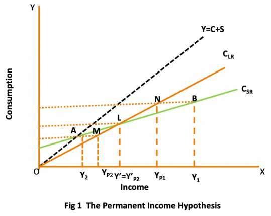
• The permanent income hypothesis is shown in Fig 1. The figure relates to a cross section of population. CLR is the long run consumption function passing through the origin. It shows that APC = MPC which is constant. This shows the proportional relationship between permanent income and permanent consumption. CSR is the short run consumption function showing non proportional relationship between measured income and measured consumption. Here short run APC >MPC and it falls as income rises and vice versa. OY’ is the average measured income. It is equal to the permanent income Y’P2. Transitory component is zero. Permanent and measured consumption at this level of income is LY’.

• Suppose the income declines to OY2. There is negative transitory income equal to Y2YP2. Consumption at this level is AY2, a rise in the APC relative to what it is at point L. Permanent income declines to OYP2. The decrease in consumption corresponding to this decrease in permanent income leads to point M from point L.

• When measured income rises to OY1, transitory income is positive. Measured income OY1, is greater than the permanent income OYP1. Consumption is BY1. APC at OY 1, will be smaller than the APC at the original level of income OY’ = ΟΥ’Ρ2.

• Thus we see that the non-proportional relationship between consumption and measured income found in the short run is based on the positive and negative transitory income component. If income were to grow at a steady rate or without cyclical variations, permanent income would be equal to measured income. Consumption would be a stable fraction of the measured income that APC would be stable rather than rising during the below average years and falling during the above average years of the business cycle.

• The long run relationship averages out the positive and negative components of transitory income in the long run, consumption is a stable function of income.

Critical Evaluation of the Permanent income Hypothesis:

• Permanent income hypothesis effects a reconciliation of the aggregate consumption functions somewhat like the relative income hypothesis. In relative income hypothesis the behavior of consumption over the business cycle is central to the reconciliation, but the key was the effect on consumption as income recedes from the previous peak income level. In the permanent income hypothesis, the key is the effect on consumption of the positive and negative transitory income component that appear as income departs from the long run path during business cycles.

The permanent income hypothesis suffers from following criticism:

1. Wrong assumptions: Friedman assumed that permanent and transitory components of income and consumption are not correlated and that transitory consumption and transitory income are uncorrelated, being independent of each other. It is asserted that a household unit is unresponsive to either a positive or negative transitory component in measured income with regard to its consumption spending behavior. The household neither reduces its consumption when its measured income in a given year falls nor does it increase its consumption expenditure when its measured income in any given year rises unexpectedly. This implies that increase or decrease in the observed or measured income are wholly saved or dis-saved. MPC out of transitory income is zero. But this is not true. When a person wins a lottery or at a race, he gives party to his friends and spends more than usual. Similarly a poor man who has lost his purse, postpones the consumption of a new coat.

2. Wrong conclusion: The conclusion that the rich and the poor spend equal fractions of their incomes on consumption is in conflict with the observed behavior of ordinary family units. This conclusion is based on the argument that savings are primarily done to even out consumption over a long period of time. But still the preference for the present goods over future goods for the low income families is not the same as it is for the high income families. At low levels of current income there is more pressure to increase the present consumption.

3. Difficulty in estimating permanent income: The concept of permanent income involves expected or anticipated income and this cannot be estimated in any direct manner. Friedman has taken permanent income of one year as a weighted average of the actual or measured income over 17 year period. Current year’s measured income was given a weight age of 33% and preceding year was assigned 22% weight age and so on for the other fifteen preceding years with the weights falling rapidly. There is however little rationale behind the weights chosen to be given to different years’ measured income for estimating the permanent income of any given year.

4. Difficulty in ascertaining the parts of aggregate measured income as permanent income and transitory income: For finding out the proper components of each year’s aggregate measured income, we require the separate data of permanent income and transitory income of every individual year. Unfortunately, no such data on an individual year basis is readily available at hand.

5. Clubbing of human and non-human wealth: Friedman’s clubbing of human and non-human forms of wealth does not seem to be justified.

6. Too much emphasis on long run planning of consumers: Friedman over emphasized the long run planning by consumers.

7. Independence of „k „of the level of income has also been questioned by many economists. According to Michael K Evans. “Friedman’s formulation has reshaped and redirected much of the research on the consumption function. It is indeed unusual to discuss the consumption function today without referring to Friedman’s terms of reference”.