

THE GOODS MARKET AND MONEY MARKET: LINKS BETWEEN THEM
Keynes explains that national income is determined at the level where aggregate demand (C + I) equals aggregate output, i.e., where the goods market is in equilibrium.
In the simple Keynesian model:
Aggregate demand consists of consumption (C) and investment (I).
National income is determined where C + I = Output.
The equilibrium level of income is thus determined in the goods market.
Investment (I) in this model:
Is determined by the rate of interest and the marginal efficiency of capital (MEC).
Is assumed to be independent of the level of national income.
The rate of interest is determined in the money market by:
The demand for money.
The supply of money.
Equilibrium in the money market.
Changes in the rate of interest (due to changes in money supply or demand for money):
Affect the level of investment.
Changes in investment affect aggregate demand (C + I).
This leads to changes in national income and output in the goods market.
Thus, money market equilibrium influences goods market equilibrium.
A criticism of the simple Keynesian model:
It appears to show only a one-way relationship.
Changes in the money market affect the goods market.
But there seems to be no reverse effect of changes in income or investment in the goods market on the money market equilibrium.
J.R. Hicks and other economists addressed this flaw:
They argued that changes in income also affect the money market.
Higher income increases the transactions demand for money.
Changes in money demand influence the rate of interest.
Therefore, there is a two-way relationship between goods and money markets.
According to Hicks:
The level of income, determined by consumption and investment, affects money demand.
Money demand influences the rate of interest.
Hence, goods market changes indirectly influence the money market.
Economists such as Hicks, Hansen, Lerner, and Johnson developed a more complete and integrated framework:
Known as the IS–LM model.
It shows the mutual interdependence of:
Investment
National income
Rate of interest
Demand for money
Supply of money
The model is represented by two curves:
The IS curve (goods market equilibrium).
The LM curve (money market equilibrium).
The IS–LM model demonstrates:
Simultaneous equilibrium in both goods and money markets.
Joint determination of national income and the rate of interest.
The IS–LM framework has become a standard tool of macroeconomics.
It is widely used to analyze the effects of monetary policy.
It is also used to examine the impact of fiscal policy.
GOODS MARKET EQUILIBRIUM : THE DERIVATION OF THE IS CURVE
The IS–LM model emphasizes the interaction between the goods market and the money market.
The goods market is in equilibrium when aggregate demand = national income.
Aggregate demand consists of:
Consumption demand (C)
Investment demand (I)
In the extended Keynesian framework:
The rate of interest is introduced as an important determinant of investment.
Investment becomes an endogenous variable.
A fall in the rate of interest leads to an increase in investment.
A rise in the rate of interest reduces investment.
Mechanism of interest affecting income:
A lower rate of interest reduces the cost of investment projects.
This raises the profitability of investment.
Businessmen undertake greater investment.
Increased investment raises aggregate demand (C + I).
Higher aggregate demand leads to a higher equilibrium level of national income.
In deriving the IS curve:
We determine equilibrium levels of national income corresponding to different rates of interest.
Each equilibrium income level is based on goods market equilibrium with investment determined by a given rate of interest.
Thus, the IS curve shows the relationship between rate of interest and equilibrium national income.
Explanation using graphical panels:
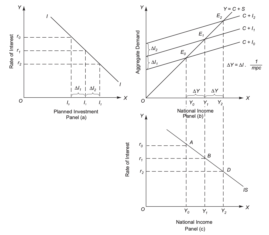
In panel (a):
The relationship between rate of interest and planned investment is shown by the investment demand curve.
At interest rate Or₀, planned investment equals OI₀.
In panel (b):
With planned investment O*I₀, aggregate demand is C + I₀.
Goods market equilibrium occurs at income level O*Y₀.
In panel (c):
The combination of Or₀ and OY₀ is plotted.
When the rate of interest falls to O*r₁:
Planned investment rises from OI₀ to OI₁.
Aggregate demand shifts upward from C + I₀ to C + I₁.
Goods market equilibrium rises to income level O*Y₁.
The combination Or₁ and OY₁ is plotted.
With a further fall in interest rate to O*r₂:
Planned investment increases to O*I₂.
Aggregate demand shifts further upward to C + I₂.
Goods market equilibrium occurs at income level O*Y₂.
The combination Or₂ and OY₂ is plotted.
By joining points representing different interest–income combinations (such as A, B, D), we derive the IS curve.
The IS curve:
Is the locus of combinations of rate of interest and national income at which the goods market is in equilibrium.
Is downward sloping (negative slope).
Indicates that a fall in the rate of interest leads to a rise in the equilibrium level of national income.
Investment and Aggregate Demand
Why does IS Curve Slope Downward?
The lower the rate of interest, the higher will be the equilibrium level of national income.
The IS curve is the locus of combinations of rate of interest and national income at which the goods market is in equilibrium.
Derivation of the IS curve (as illustrated in Fig. 12.1):
In panel (a):
The relationship between rate of interest and planned investment is shown by the investment demand curve (II).
At interest rate Or₀, planned investment equals OI₀.
In panel (b):
With planned investment OI₀, the aggregate demand curve becomes C + I₀.
Aggregate demand equals aggregate output at income level OY₀.
Thus, the goods market is in equilibrium at OY₀.
In panel (c):
The combination of Or₀ (interest rate) and OY₀ (income level) is plotted.
When the rate of interest falls to Or₁:
Planned investment increases from OI₀ to OI₁ (panel a).
The aggregate demand curve shifts upward from C + I₀ to C + I₁ (panel b).
Goods market equilibrium rises to income level OY₁.
The combination Or₁ and OY₁ is plotted in panel (c).
With a further fall in the rate of interest to Or₂:
Planned investment increases to OI₂ (panel a).
Aggregate demand shifts upward to C + I₂ (panel b).
Goods market equilibrium occurs at income level OY₂.
The combination Or₂ and OY₂ is plotted in panel (c).
By joining points A, B, and D representing different interest–income combinations, the IS curve is obtained.
The IS curve:
Is downward sloping (negative slope).
Shows an inverse relationship between rate of interest and equilibrium national income.
Implies that a decline in the rate of interest leads to an increase in the equilibrium level of national income.
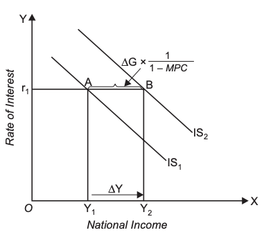
in Government Expenditure