
Consumer Behaviour
- Consumer Behaviour is the study of how individual customers, groups or organizations select, buy, use, and dispose ideas, goods, and services to satisfy their needs and wants. It refers to the actions of the consumers in the marketplace and the underlying motives for those actions.
- The study of consumer Behaviour assumes that the consumers are actors in the marketplace. The perspective of role theory assumes that consumers play various roles in the marketplace. Starting from the information provider, from the user to the payer and to the disposer, consumers play these roles in the decision process.
- Consumer Behaviour is a complex , dynamic, Multidimensional process and all marketing decisions are based on the assumptions about consumer Behaviour which includes communicating , Purchasing , and consuming , interacting.
Meaning and Definition
- Consumer Behaviour is the study of how individual customers, groups or organizations select, buy, use, and dispose ideas, goods, and services to satisfy their needs and wants. It refers to the actions of the consumers in the marketplace and the underlying motives for those actions.
- In the words of Engel, Blackwell, and Mansard, “consumer Behaviour is the actions and decision processes of people who purchase goods and services for personal consumption”.
- According to Schiffman “Consumer Behaviour is defined as Behaviour that consumers display in searching for purchasing, using evaluating and disposing of products and services that expect will satisfy their needs”.
- According to Louden and Bitta, “Consumer Behaviour is the decision process and physical activity, which individuals engage in when evaluating, acquiring, using or disposing of goods and services”.
Nature of Consumer Behaviour
- Influenced by Various Factors:
- Marketing factors such as product design, price, promotion, packaging, positioning and distribution.
- Personal factors such as age, gender, education and income level.
- Psychological factors such as buying motives, perception of the product and attitudes towards the product.
- Situational factors such as physical surroundings at the time of purchase, social surroundings and time factor.
- Social factors such as social status, reference groups and family.
- Cultural factors, such as religion, social class—caste and sub-castes.
- Undergoes a constant change: Consumer Behaviour is not static. It undergoes a change over a period of time depending on the nature of products.
- Varies from consumer to consumer: All consumers do not behave in the same manner. Different consumers behave differently. The differences in consumer Behaviour are due to individual factors such as the nature of the consumers, lifestyle and culture.
- Varies from region to region and country to county: The consumer Behaviour varies across states, regions and countries. It may differ depending on the upbringing, lifestyles and level of development.
- Information on consumer Behaviour is important to the marketers: Marketers need to have a good knowledge of the consumer Behaviour. They need to study the various factors that influence the consumer Behaviour of their target customers. i.e. Product design/model, pricing, packaging, positioning, promotion of product etc…
- Leads to purchase decision: A positive consumer Behaviour leads to a purchase decision. A consumer may take the decision of buying a product on the basis of different buying motives. The purchase decision leads to higher demand, and the sales of the marketers increase.
- Varies from product to product: Consumer Behaviour is different for different products. There are some consumers who may buy more quantity of certain items and very low or no quantity of other items.
- Improves standard of living: The buying Behaviour of the consumers may lead to higher standard of living. The more a person buys the goods and services, the higher is the standard of living. But if a person spends less on goods and services, despite having a good income, they deprives themselves of higher standard of living.
- Reflects status: The consumer Behaviour is not only influenced by the status of a consumer, but it also reflects it. The consumers who own luxury products like luxury car, watches and other items are considered belonging to a higher status. The luxury items also give a sense of pride to the owners.
Consumer
A Consumer is an individual who buys products or services for personal use and not for manufacture or resale . A Consumer may be a person or group of people such as a household and similar needs, not directly related to entrepreneurial or business activities who are the final users of products or services. Consumers are the basic economic entities of an economy. All the consumers consume goods and services directly and indirectly to maximise satisfaction and utility.
Types of Consumer:
- Personal Consumer/ Individual consumer: Buy the Product and services for his family and own or family.
- Organizational Consumers/Commercial consumers: Buy the product or services for manufacturing or reselling.
Importance of Studying Consumer Behaviour
- Modern Philosophy: It concerns with modern marketing philosophy – identify consumers’ needs and satisfy them more effectively than competitors. It makes marketing consumer-oriented. It is the key to succeed.
- Achievement of Goals: The key to a company’s survival, profitability, and growth in a highly competitive marketing environment is its ability to identify and satisfy unfulfilled consumer needs better and sooner than the competitors. Thus, consumer Behaviour helps in achieving marketing goals.
- Useful for Dealers and Salesmen: The study of consumer Behaviour is not useful for the company alone. Knowledge of consumer Behaviour is equally useful for middlemen and salesmen to perform their tasks effectively in meeting consumers needs and wants successfully. Consumer Behaviour, thus, improves performance of the entire distribution system.
- More Relevant Marketing Programme: Marketing programme, consisting of product, price, promotion, and distribution decisions, can be prepared more objectively. The programme can be more relevant if it is based on the study of consumer Behaviour. Meaningful marketing programme is instrumental in realizing marketing goals.
- Adjusting Marketing Programme over Time: Consumer Behaviour studies the consumer response pattern on a continuous basis. So, a marketer can easily come to know the changes taking place in the market. Based on the current market trend, the marketer can make necessary changes in marketing programme to adjust with the market.
- Predicting Market Trend: Consumer Behaviour can also aid in projecting the future market trends. Marketer finds enough time to prepare for exploiting the emerging opportunities, and/or facing challenges and threats.
- Consumer Differentiation: Market exhibits considerable differentiations. Each segment needs and wants different products. For every segment, a separate marketing programme is needed. Knowledge of consumer differentiation is a key to fit marking offers with different groups of buyers. Consumer Behaviour study supplies the details about consumer differentiations.
- Creation and Retention of Consumers: Marketers who base their offerings on a recognition of consumer needs find a ready market for their products. Company finds it easy to sell its products. In the same way, the company, due to continuous study of consumer Behaviour and attempts to meet changing expectations of the buyers, can retain its consumers for a long period.
- Competition: Consumer Behaviour study assists in facing competition, too. Based on consumers’ expectations, more competitive advantages can be offered. It is useful in improving competitive strengths of the company.
- Developing New Products: New product is developed in respect of needs and wants of the target market. In order to develop the best-fit product, a marketer must know adequately about the market. Thus, the study of consumer Behaviour is the base for developing a new product successfully.
- Dynamic Nature of Market: Consumer Behaviour focuses on dynamic nature of the market. It helps the manager to be dynamic, alert, and active in satisfying consumers better and sooner than competitors. Consumer Behaviour is indispensable to watch movements of the markets.
- Effective Use of Productive Resources: The study of consumer Behaviour assists the manager to make the organisational efforts consumer-oriented. It ensures an exact use of resources for achieving maximum efficiency. Each unit of resources can contribute maximum to objectives.
Factors Influencing Consumer Behaviour
The behaviour of consumer is dependent on a number of factors which may be economic or non-economic factors and are dependent upon economic factors such as income, price, psychology, sociology, anthropology, culture and climate. The study of consumer behaviour has proved that following are the main factors which influence the behaviour:
- Economic Factors: Price, Income, Distribution of Income, Competition with substitute , utility and Consumer preferences are the factors categorised as Economic factors .
- Social Factors: Culture, Attitude of society, social values, Life-style, personality, Size of family, Education, health standards are the factors catagorised as Social factors.
- Psychology : It decides the personality, taste, attitudes of individuals or groups, life style, preferences especially on occasions like marriage. The demonstration influence is also dependent upon psychology of an individual.
- Anthropology & Geography: Climate, region, history all effect, consumer behaviour. In hot countries like India certain products which keep us cool like squashes, sarbatas, are demanded but they have no demand in cold regions. Culture is also influenced by climate.
- Technology: In case of equipment’s whether for consumer use or industrial use is affected by technological innovations and features. Even in case of perishable goods the shelf life etc are determined by technological developments. Innovations and introduction of new product also depends upon technological development.
- Others: Knowledge-technical or otherwise and information. Government decisions, laws, distribution policies, production policies have also big affect on consumer behaviour.
Advantages of Study of Consumer Behaviour
- Saves from Disaster: The failure rate of new products is surprisingly high not only in highly competitive economies of USA, Europe and Japan etc. but even in India. For instance, Roohafza of Hamdard succeeded well but when other companies tried like Dabur to produce similar products they could not succeed. There are many more such examples. If one tests the market before launching a new product this type of disaster can be avoided or minimized.
- Helps in Formulating Right Marketing Strategy: If one studies well what factors will influence demand of a product accordingly production and marketing strategies can be framed. In food items it is taste which decides whether consumer will buy it or not. If through the study of consumer behaviour one is able to know correctly the factors which influence buying decisions of the consumer one can promote sales of existing or new product.
- Segmentation of Market is Helped: The study of consumer behaviour suggested that everyone does not buy on price consideration or utility consideration only. For high income group’s high priced cloth, cars, etc have been produced. The producers of such items make heavy profits which would not have been possible without study of consumer behaviour because it is against basic economic theory.
- Helps in Development of New Products: Before launching a new product proper study of consumer tastes i.e. behaviour avoids later failure and loss. This is particularly true for food items and daily consumption products. It is equally true for fashion goods like garments, cosmetics, cigarettes and new flavors of existing products. In certain cases if a product is reintroduced after a long gap this type of study helps.
- Helps in Product Orientation: The study of consumer behaviour helps to find-out why consumers are drifting away from a product or why they are not liking it. For instance, some of Indian toothpastes are being produced for long like Neem but it could not capture the market. There are many other instances when a new product has been developed or reoriented to again capture its old glorious position. Those who do it scientifically succeed and others who do not study consumer behaviour properly or do not orient loose the market, merely by pretty faces or fancy claims he wants to be assured that what is claimed is really true.
- Helps in Reorientation of Packaging: A great deal of importance is being given to packaging for quite some time by marketing department and market research. But whether a particular packaging is liked by consumers or not is a recent phenomenon. Consumer if likes a packing helps in pushing sales. In certain cases this fact is advertised also. But in many cases this has been done without study of consumer behaviour and his attraction or disliking of a particular packaging. The fact however remains that proper study can help in pushing sales.
- Helps Consumers to Study their Behaviour: The consumers often are guided by their income, emotions, opinion of others and they do not undertake study of their behaviour whether it is scientific or not. The science, however, can help them to study cost benefit of their buying decisions. The study can reveal them whether buying an expansive item is rational, or not. If there are competitive goods it can help them to make consumer preference chart and then decide what to buy immediately and what to postpone and what should be rejected.
Limitations of Study of Consumer Behaviour
Consumer buying behavior relates to the identification of consistent stages of decision making used in every purchase situation. The process begins with need recognition, followed by information gathering, a purchase and finally, post-purchase evaluation. Marketers rely on an understanding of buyer behavior to effectively position products and services.
However, consumer buying behavior does have following limitations:
- Inconsistency: One of the biggest drawbacks of relying too heavily on consumer buying behavior is that consumers rarely apply the same steps in the same way for every product and service purchase. This makes it more difficult for marketers trying to stimulate a need or to offer messages that enhance the likelihood of a purchase for their brand. Thus, most companies have to perform more research into their particular market segments and how they approach their brand.
- Limited Buyer Interest: Another primary limitation for marketers using the consumer buying behavior model is that consumers sometimes are much less involved in a purchase decision. For instance, someone buying laundry detergent is generally less involved in the purchase than someone buying a car or washer and dryer. Thus, the ability of marketers to affect consumers by analyzing buyer behavior is limited.
- Social and Cultural Influences: Marketers spend significant time trying to interpret consumer buying behavior related to their products, but they must also understand how each given customer is influenced externally by social relationships and culture. However, knowing how a given customer is influenced by family, friends and their community for purchases of appliances, food and household items is significantly more complex.
- Applying Stimuli: In its “Buyer Behavior” overview, MMC Learning points out that marketing tries to respond to consumer buying behavior by communicating with stimuli expected to elicit the desired consumer response. Unfortunately, MMC Learning notes that buying behavior involves a number of complicated psychological variables related to consumer perception, motivation, learning, memory, attitude and personality. Accurately predicting response to a given message often demands significant marketing research and focus group studies.
Demand
- Economics is a study of market that comprise a group of buyers and seller of a particular product or service. The working of the market system is governed by two forces, demand and supply. These two forces play a crucial role in determining the price of a product and size of the market.
- Demand is the rate at which consumers want to buy a product. Economic theory holds that demand consists of two factors: taste and ability to buy. Taste, which is the desire for a good, determines the willingness to buy the good at a specific price. Ability to buy means that to buy a good at specific price, an individual must possess sufficient wealth or income.
- Demand refers to the willingness as well as ability of a buyer to pay for a particular product. In other words, demand can be defined as the quantity of a product that a buyer desires to purchase at a specific price and time period. The demand for a product is influenced by a number of factors, such as price of the product, change in customers’ preferences and standard of living.
- The demand for a product in the market is governed by the law of demand, which states that the demand for a product decreases with increase in its prices and vice versa, while other factors are constant. In the market system, buyer constitute the demand for a product, while sellers represent the supply side of the product in the market.
Concept of Demand
Theoretically, demand can be defined as a quantity of a product an individual is willing to purchase at a specific point of time. Some of the management experts have defined demand in the following ways:
- “The demand for anything, at a given price is the amount of it which will be bought per unit of time at the price.” – Prof. Benham
- “By demand is meant, demand at a price, for it is impossible to conceive of demand not related to price.” – Prof. Hanson
- “Demand means the various quantities of goods that would be purchased per time period at different prices in a given market.” – Prof. Hibdon
- “The demand for goods is schedule of the amounts that buyers would be willing to purchase at all possible prices at any one instant of time.” – Prof. Mayers
- From the aforementioned definitions, it can be concluded that demand implies a desire supported by an ability and willingness of an individual to pay for a particular product. If an individual does not have sufficient resources or purchasing power to buy a particular product, then his/her desire alone would not be regarded as demand.
- For instance, if an individual desires to purchase a Ferrari Car and does not have adequate amount of money to purchase the car, his/her desire is not considered as demand for the car.
- Apart from it, if an affluent individual desires to purchase a car, but does not have willingness to spend money for purchasing the car then his/her desire is also not considered as demand.
- Therefore, we can say that effective demand is the desire backed by the purchasing power and willingness of an individual to pay for a particular product. An effective demand has three characteristics namely, desire, willingness, and ability of an individual to pay for a product.
- The demand for a product is always defined in reference to three key factors—price, point of time, and market place. These three factors contribute a major part in understanding the concept of demand. The omission of any of these factors would make the concept of demand meaningless and vague.
Demand Analysis
- Demand analysis is a research done to estimate or find out the customer demand for a product or service in a particular market. Demand analysis is one of the important consideration for a variety of business decisions like determining sales forecasting, pricing products/services, marketing and advertisement spending, manufacturing decisions, expansion planning etc.
- Demand analysis covers both future and retrospective (iwo±O;kih) analysis so that they can analyze the demand better and understand the product/service’s past success and failure too.
- For a new company, the demand analysis can tell whether a substantial demand exists for the product/service and given the other information like number of competitors, size of competitors, industry growth etc it helps to decide if the company could enter the market and generate enough returns to sustain and advance its business.
- Demand analysis helps in identifying key business areas where demand is highest and areas which needs attention as very low demand indicates different problems like either the customers are not aware of the product/service and more focus must be in advertisement and promotion or the customer needs are not met by current product/service and improvements are needed or competitors have sprung up with better offerings etc.
Significance of Demand
The demand analysis is of crucial importance to the business enterprises. It is the source of many useful insights for business decision making. The success or failure of business firms depend primarily on its ability to generate resources by satisfying the demand of consumers. The firms unable to attract consumers are soon forced out from the market. The importance of demand analysis in business decisions can be explained under following headings:
- Sales Forecasting: The demand is a basis for the sales of the production of a firm. Hence, sales forecasting can be made on the basis of demand. For example, if demand is high, sales will be high and if demand is low, sales will also be low. The firms can make different arrangements to increase or reduce production or push up sales on the basis of sales forecast.
- Pricing Decisions: The analysis of demand is the basis of pricing decisions of a firm. If the demand for the product is high, the firm can charge high price, other things remaining the same. On the contrary, if the demand is low, the firm cannot charge high price. The demand analysis also helps the firm in profit budgeting.
- Marketing Decisions: The analysis of demand helps a firm to formulate marketing decisions. The demand analysis analyses and measures the forces that determine demand. The demand can be influenced by manipulating the factors on which consumers base their demand on attractive packaging.
- Production Decisions: How much a firm can produce depends on its capacity. But how much it should produce depends on demand. Production is not necessary if there is no demand. But continuous production schedule is necessary if the demand for the production is relatively stable. If the demand is less than the quantity of production, new demand should be created by means of promotional activities such as advertising.
- Financial Decisions: The demand condition in the marker for firm’s product’s affects the financial decisions as well. If the demand for firm’s product is strong and growing, the needs for additional finance will be greater. Hence, the financial manager should make necessary financial arrangement to finance the growing needs of the capital.
Law of Demand
Introduction
- The law of demand is one of the most fundamental concepts in economics. It works with the law of supply to explain how market economies allocate resources and determine the prices of goods and services that we observe in everyday transactions.
- The law of demand states that quantity purchased varies inversely with price. In other words, the higher the price, the lower the quantity demanded. This occurs because of diminishing marginal utility. That is, consumers use the first units of an economic good they purchase to serve their most urgent needs first, and use each additional unit of the good to serve successively lower valued ends.
Meaning
- Economics involves the study of how people use limited means to satisfy unlimited wants. The law of demand focuses on those unlimited wants. Naturally, people prioritize more urgent wants and needs over less urgent ones in their economic behaviour, and this carries over into how people choose among the limited means available to them. For any economic good, the first unit of that good that a consumer gets their hands on will tend to be put to use to satisfy the most urgent need the consumer has that that good can satisfy.
- For example, consider a castaway on a desert island who obtains a six pack of bottled, fresh water washed up on shore. The first bottle will be used to satisfy the castaway’s most urgently felt need, most likely drinking water to avoid dying of thirst. The second bottle might be used for bathing to stave off disease, an urgent but less immediate need. The third bottle could be used for a less urgent need such as boiling some fish to have a hot meal, and on down to the last bottle, which the castaway uses for a relatively low priority like watering a small potted plant to keep him company on the island.
- In our example, because each additional bottle of water is used for a successively less highly valued want or need by our castaway, we can say that the castaway values each additional bottle less than the one before. Similarly, when consumers purchase goods on the market each additional unit of any given good or service that they buy will be put to a less valued use than the one before, so we can say that they value each additional unit less and less. Because they value each additional unit of the good less, they are willing to pay less for it. So the more units of a good consumers buy, the less they are willing to pay in terms of the price.
Important Facts:
The law of demand is a fundamental principle of economics which states that at a higher price consumers will demand a lower quantity of a good.
Demand is derived from the law of diminishing marginal utility, the fact that consumers use economic goods to satisfy their most urgent needs first.
A market demand curve expresses the sum of quantity demanded at each price across all consumers in the market.
Changes in price can be reflected in movement along a demand curve, but do not by themselves increase or decrease demand.
The shape and magnitude of demand shifts in response to changes in consumer preferences, incomes, or related economic goods, NOT to changes in price.
Demand and Supply
Introduction
Market mechanism plays a crucial role in solving the basic economic problems of a free market economy and that the entire market system functions in an orderly manner, though some aspects of it may not be desirable. The market system functions in an orderly manner because it works under certain fundamental laws of market known as the laws of demand and supply.
Conceptually, demand can be defined as the desire to buy a good for which the demander has ability and willingness to pay. In simple words, demand is a desire for a good, backed by ability and willingness to pay. A desire without ability to pay is merely a wish. A desire with ability to pay but without willingness to pay is only a potential demand. A desire accompanied by ability and willingness to pay makes a real or effective demand.
Supply side of the market refers to the sellers of a product in the market. Supply is the quantity supplied at a given price per unit of time.
Law of Demand its Exceptions
For the purpose of demand analysis, a distinction is often made between the individual demand and the market demand—individual demand for analysing consumer behaviour and market demand for analysing market behaviour.
Individual demand refers to the quantity of a commodity that a person is willing to buy at a given price over a specified period of time, say per day, per week, per month, etc.
Market demand refers to the total quantity that all the users of a commodity are willing to buy at a given price over a specific period of time. In fact, market demand is the sum of individual demands for a product.
The Law of Demand:
The law of demand states the relationship between the quantity demanded and the price of a commodity. In general, quantity demanded of a commodity depends on many other factors also, viz., consumer’s income, price of the related goods (substitutes and complements), consumer’s taste and preferences, advertisement, etc. However, price of a product is the most important and the only determinant of its demand in the short run because other factors are taken to remain constant. Therefore, the law of demand is linked to the price of the product.
The law of demand can be stated as ‘all other things remaining constant, the quantity demanded of a commodity increases when its price decreases and demand decreases when its price increases’. This law implies that demand and price are inversely related. Marshall states the law of demand as ‘the amount demanded increases with a fall in price and diminishes with a rise in price’. This law holds under ceteris paribus assumption, i.e., all other determinants of demand remain unchanged. The law of demand can be illustrated through a demand schedule and a demand curve.
The Demand Schedule
A demand schedule is a tabular presentation of quantity demanded of a commodity at different prices per unit of time. A hypothetical market demand schedule is given in Table below. This table presents price of shirts (Ps ) and the corresponding number of shirts demanded (Qs ) per month.
Table 1. Demand Schedule for Shirts
| Pₛ (Price in ₹) | Qₛ (Shirts in ’000) |
|---|---|
| 800 | 8 |
| 600 | 15 |
| 400 | 30 |
| 300 | 40 |
| 200 | 55 |
| 100 | 80 |
Table above illustrates the law of demand. As data given in the table shows, the demand for shirts (Qs ) increases as its price (Ps ) decreases. For instance, at price 800 per shirt, only 10,000 shirts are demanded per month. When price decreases to 400, the demand for shirts increases to 30,000 and when price falls further to 100, demand rises to 80,000. Similarly, one can read the table in reverse order and arrive at the conclusion that as price of shirt increases, its demand decreases. This relationship between the price and the quantity demanded gives the law of demand.
The Demand Curve
A demand curve is a graphical presentation of the demand schedule. For example, when the data given in the demand schedule (Table 1) are presented graphically as shown in Figure 1, the resulting curve DD’ represents the demand curve.
The curve DD’ in Figure 1 depicts the law of demand. It slopes downward to the right. That is, it has a negative slope.
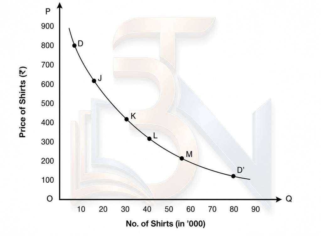
Fig 1. The Demand Curve
The negative slope of the demand curve DD’ shows the inverse relationship between the price of shirt and its quantity demanded. The inverse relationship means that demand increases with the decrease in price and decreases with the rise in price.
As can be seen in Figure 1, downward movement on the demand curve DD’ from point D towards D’ shows fall in price and rise in demand. Similarly, an upward movement from point D’ towards D reads rise in price and fall in demand.
The law of demand is based on an empirical fact, i.e., based on real market data. For example, when prices of cell phones and personal computers (PCs), especially of the latter, were astronomically high, only few rich persons and big firms could afford them. Now with the revolution in computer and cell phone technology and the consequent fall in their prices, demand for these goods has shot up in India though other factors too contributed to rise in demand for these goods.
The Factors Behind the Law of Demand
According to the law of demand, when a price of a product increases, its demand decreases and vice versa, all other demand determinants remaining constant. A question arises here: what are the factors behind the law of demand or why does demand decrease when price rises or other way round? The factors behind the law of demand are the following.
Income effect: When price of a commodity falls, purchasing power of the consumers increases since they are required to pay less for the same quantity. According to another economic law, increase in real income (or purchasing power) increases demand for the goods and services in general and for the goods with reduced price in particular. The increase in demand on account of increase in real income is called income effect.
It should, however, be noted that the income effect is negative in case of inferior goods. In case, price of an inferior good accounting for a considerable proportion of the total consumer expenditure falls substantially, consumers’ real income increases. Consequently, they substitute superior goods for inferior ones. Therefore, income effect on the demand for the inferior good becomes negative.
Substitution effect: When price of a commodity falls, it becomes cheaper compared to its substitutes, prices of substitutes remaining constant. In other words, when price of a commodity falls, price of its substitutes remaining the same, its substitutes become relatively costlier. Consequently, rational consumers tend to substitute cheaper goods for costlier ones within the range of normal goods—goods whose demand increases with the increase in consumer’s income—other things remaining the same. Therefore, demand for the relatively cheaper goods increases. The increase in demand on account of substitution of cheaper good for the relatively costlier one is known as substitution effect.
Diminishing marginal utility: Marginal utility is the utility derived from the marginal unit consumed of a commodity. Diminishing marginal utility is also responsible for the increase in demand for a commodity when its price falls. When a person buys a commodity, he exchanges his money income with the commodity in order to maximize his satisfaction. The utility of money is assumed to remain constant and utility of money is equal to price paid. Under this condition, a consumer continues to buy goods and services so long as marginal utility of his money \((MU_m)\) is less than the marginal utility of the commodity \((MU_c)\). Given the price \((P_c)\) of a commodity, the consumer adjusts his purchases so that \((MU_c = MU_m)\). When the price of commodity decreases, the utility of money hence to be higher than the product. A utility maximizing consumer spends more money to attain equilibrium at \((MU_c = MU_c)\). This fact increases the demand with decrease in the price.
Exceptions to the Law of Demand (Giffen Goods)
The law of demand is one of the fundamental laws of economics. The law of demand, however, does not apply under the following cases.
Expectations regarding future prices: When consumers expect a continuous increase in the price of a durable commodity, they buy more of it despite the increase in its price just to avoid the pinch of still higher price in future. Similarly, when consumers anticipate a considerable decrease in the price in future, they postpone their purchases and wait for the price to fall further, rather than buy the commodity when its price initially falls. Such decisions of the consumers are contrary to the law of demand.
Prestigious goods: The law of demand does not apply to the commodities which are used as a ‘status symbol’. Prestige goods are the goods which enhance social prestige or display wealth and richness, e.g., gold, precious stones, rare paintings and antiques. Rich people buy such goods mainly because their prices are high.
Giffen goods: A classic exception to the law of demand is the case of Giffen goods named after a British economist, Sir Robert Giffen (1837–1910). A Giffen good does not mean any specific commodity. It may be any inferior but essential commodity much cheaper than its substitutes, consumed mostly by the poor households and claiming a large part of their income. If the price of such goods increases (price of its substitute remaining constant), its demand increases instead of decreasing.
For instance, let us suppose that the monthly minimum consumption of food grains by a poor household is 30 kg including 20 kg of bajra (an inferior good) and 10 kg of wheat (a superior good). Suppose also that bajra sells at ₹5/kg and wheat at ₹10/kg. At these prices, the household spends ₹200 per month on food grains. That is the maximum it can afford.
Now, if price of bajra increases to ₹6 per kg, the household will be forced to reduce its consumption of wheat by 5 kg and increase that of bajra by the same quantity in order to meet its minimum monthly consumption requirement within ₹200 per month. Obviously, household’s demand for bajra increases from 20 to 25 kg per month despite increase in its price and that of wheat falls to 5 kg.
Elasticity of Demand, Price, Income and Cross
Before we proceed to discuss the elasticity of demand, let us have a clear view of the components of demand elasticities. The demand for a product, especially in the long run, depends on several factors as listed below.
Price of the product,
Consumers’ income;
Price of substitutes and complements;
Advertisement of the product;
Future price expectations; and
Consumers’ taste and fashion.
Of these demand determinants, the effect of change in consumers’ taste and fashion is difficult to quantify. In practice, therefore, the overall demand for a product is generally deemed to be determined by the quantifiable demand determinants, viz., price of the product, consumers’ income, price of the substitutes and compliments, ad-spending by the firms and consumers’ expectations about the future prices. Therefore, the overall demand and change in demand for a product depends on the nature and extent of change in these demand determinants. And, the overall elasticity of demand for a commodity depends on the combined effects of changes in these demand determinants.
Therefore, the elasticity of demand is measured separately with respect to all its major determinants. Following this practice, we discuss in this unit, the following kinds of demand elasticities.
Price elasticity of demand;
Income elasticity of demand; and
Cross-elasticity of demand, i.e., demand elasticity with reference to price of substitutes and complementary goods.
All these kinds of demand elasticities are discussed in this chapter. However, of these kinds of elasticities of demand, price elasticity of demand is of the greatest significance from both theoretical and practical points of view.
The Price Elasticity of Demand
The price elasticity of demand is defined as the degree of responsiveness of demand for a commodity to the change in its price. The price elasticity of demand, i.e., the responsiveness of demand for a commodity to change in its price, is measured as the percentage change in the quantity demanded divided by the percentage change in the price. That is, \((e_p = \frac{\text{Percentage change in the quantity demanded}}{\text{Percentage change in the price}})\). Here, \((e_p)\) denotes the price elasticity of demand. The numerical value of \((e_p)\) is called the coefficient of demand elasticity.
A general formula for measuring the price elasticity of demand is derived as follows. Here, \((Q_1)\) = original demand, \((Q_2)\) = demand after price change, \((P_1)\) = original price and \((P_2)\) = changed price. By denoting \((Q_2 – Q_1)\) as \((\Delta Q)\) and \((P_2 – P_1)\) as \((\Delta P)\), a general formula for measuring price elasticity coefficient is expressed as follows:
$$(e_p = \frac{\left(\frac{\Delta Q}{Q_1}\right)}{\left(\frac{\Delta P}{P_1}\right)})$$
or,
$$(e_p = \frac{\Delta Q}{\Delta P} \times \frac{P_1}{Q_1}) (2.1)$$
To measure price elasticity of demand numerically by using the formula \((e_p = \frac{\Delta Q}{\Delta P} \times \frac{P_1}{Q_1})\) given in Eq. (2.1), let us suppose that price of a commodity X and its demand at two different prices are given in Table 2. Given the price-quantity data, \((\Delta P)\) and \((\Delta Q)\) can be worked out as:
\((\Delta P = 8 – 10 = -2)\)
\((\Delta Q = 60 – 50 = 10)\)
Therefore, the price elasticity coefficient is calculated as:
$$(e_p = \frac{\left(\frac{Q_2 – Q_1}{Q_1} \times 100\right)}{\left(\frac{P_2 – P_1}{P_1} \times 100\right)} = \frac{\left(\frac{Q_2 – Q_1}{Q_1}\right)}{\left(\frac{P_2 – P_1}{P_1}\right)})$$
Table 2: Price of Commodity X and Quantity Demanded
| Price of X (₹) | Quantity Demanded |
|---|---|
| 10 | 50 |
| 8 | 60 |
- By substituting these values in elasticity formula as given in Eq. (2.1), we get: \(e_p = – \frac{10}{-2} \times \frac{10}{50} = 1\). Thus, elasticity coefficient (\(e_p\)) equals 1.
- Note that a minus sign (\(-\)) is inserted in the formula for measuring elasticity with a view to making elasticity coefficient a non-negative value. The coefficient of price elasticity calculated without minus sign in the formula will always be negative, because either \(P\) or \(Q\) will carry a negative sign depending on whether price increases or decreases. But a negative coefficient of elasticity is rather misleading because elasticity cannot be negative—less than zero. The minus sign is, therefore, inserted in the price elasticity formula as a matter of ‘linguistic convenience’ to make the coefficient of elasticity a non-negative value.
- Sometimes, it is also advised to ignore the negative sign of \(P\) or \(Q\). The price elasticity measure is, however, always reported with a negative sign just to indicate inverse relationship between the price change and the quantity demanded.
The Arc and Point Elasticity:
When price elasticity of demand is measured between any two finite points on a demand curve, it is called arc elasticity and elasticity measured at a point on the demand curve is called point elasticity.
As noted above, price elasticity of demand is measured as the percentage change in the quantity demanded due to a certain percentage change in price. The percentage change in price may be considerably high (e.g., 20 per cent or even higher) or it may be very small—so small that it is not significantly different from zero.
When change in price is significantly high, it shows a movement from one point on the demand curve to another point, making an arc. Therefore, the price elasticity measured for a considerably high change in price is called arc elasticity of demand.
And, when price elasticity is measured for very small changes in price—not significantly different from zero—it is called point elasticity.
Method of Measuring Arc Elasticity:
As noted above, the arc elasticity of demand is the measure of elasticity between any two finite points on the demand curve. Suppose a demand function for commodity X is given as:
\(Q_x = 80 – 2P_x\)
The price quantity data generated by this demand function presented graphically, produces the demand curve, PM, as shown in Figure 2.
The measure of elasticity between any two points on the demand curve PM gives the arc elasticity. For example, the measure of the price elasticity of demand between points J and K on the demand curve PM in Figure 2 is the measure of arc elasticity. The movement from point J to K on the demand curve PM shows a fall in price of commodity X from 25 to 15 and the consequent increase in demand from 30 to 50 units.
Here,
\(\Delta P = 15 – 25 = -10\)
\(\Delta Q = 50 – 30 = 20\)
The arc elasticity between points J and K (moving from J to K) can be measured by using the formula given in Eq. (2.1), as given below:
\(\displaystyle e_p=\frac{\Delta Q}{\Delta P}\times\frac{P}{Q}\)
where P and Q are the original price and the original quantity demanded, respectively. (2.2)
\(\displaystyle e_p=\frac{-20}{-10}\times\frac{25}{30}=1.66\)
Point Elasticity is the measure of price elasticity at a finite point on a demand curve. However, as ‘point’ is defined in geometry, it occupies no space and has no dimensions. It implies that there is no change in the price and hence no change in the quantity demanded. Therefore, the concept of ‘point elasticity’ may not appear to be reasonable. However, from practical point of view, point elasticity concept is applied to an insignificant change in the price and the consequent change in the quantity demanded. Point elasticity is, in fact, the measure of the proportionate change in the quantity demanded in response to a very small proportionate change in the price. The concept of point elasticity is useful where change in the price and the consequent change in the quantity demanded are infinitesimally small. Besides, it offers an alternative to the arc elasticity. Point elasticity may be symbolically expressed as:
\(\displaystyle e_p=\frac{\partial Q}{\partial P}\times\frac{P}{Q}\) (2.3)
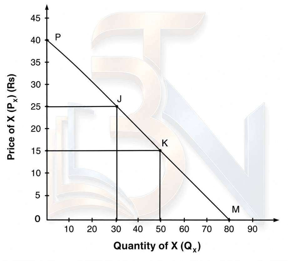
Fig 2. Change in Price and Arc Elasticity Coefficient
Determinants of Price Elasticity of Demand:
The price elasticity of demand varies from commodity to commodity depending on the nature of the commodity. While the demand for some commodities is highly elastic, for some it is highly inelastic. Besides, given the nature of a commodity, there are several other factors which determine the price elasticity of demand for a commodity. The effect of the main determinants of the price elasticities of demand is described in this section.
Availability of substitutes: One of the most important determinants of price elasticity of demand for a commodity is the availability of its substitutes. The closer the substitute, the greater the price elasticity of demand for a commodity. For instance, coffee and tea may be considered as close substitutes for one another. If price of one of these goods (say, coffee) increases, then the demand for coffee decreases more heavily. The reason is that the other commodity (tea) becomes relatively cheaper. Therefore, consumers buy more of the relatively cheaper good (tea) and less of the costlier one. Besides, the wider the range of the substitutes, the greater the elasticity. For instance, soaps, toothpastes, cigarettes, etc. are available in different brand names, each brand being a close substitute for the other, all other things remaining the same. Therefore, the price elasticity of demand for each brand will be much greater than the generic commodity. On the other hand, sugar and salt do not have their close substitute and hence their price elasticity is lower.
Nature of commodity: Price elasticity of demand depends also on the nature of a commodity. Commodities can be grouped broadly as luxuries, comforts and necessities, on the basis of the degree of intensity of the need they satisfy.
Demand for luxury goods (e.g., air conditioners, costly TV sets, cars, and decoration items) is more elastic than the demand for other kinds of goods because consumption of luxury goods can be postponed when their price rises.
On the other hand, consumption of necessities (e.g., sugar, clothes, vegetables, electricity, medicines) cannot be postponed and hence their demand has lower inelasticity.
Demand for comforts is generally more elastic than that for necessities and less elastic than the demand for luxuries.
Commodities may also be classified as durable goods and non-durable goods. Demand for durable goods is more elastic than that for non-durable goods—mainly necessities because when the price of the former increases, people either get the old one repaired instead of replacing it or buy a ‘second-hand’.
Proportion of income spent: Another factor that influences the elasticity of demand is the proportion of consumer’s income spent on a particular commodity. If proportion of income spent on a commodity is very small, its demand will be inelastic, and vice versa. Classic examples of such commodities are salt, sugar, books, toothpastes, which claim a very small proportion of consumers’ income. Demand for these goods is generally inelastic because increase in the price of such goods does not substantially affect consumer’s budget.
Time factor: Price elasticity of demand for high-price goods depends also on the time consumers can take to adjust their consumption expenditure to buy a new commodity—the shorter the time taken, the greater the elasticity. Consumers are able to adjust their expenditure pattern to price changes over a short period of time. For instance, if price of TV sets is decreased, demand will immediately increase if people possess excess purchasing power and require a short time to take decision. But, if not, then people may not be able to adjust their expenditure pattern over a short period of time to buy a TV set at the (new) lower price. If consumption adjustment takes a long period, it creates uncertainty and makes elasticity lower.
Range of alternative uses of a commodity: The wider the range of alternative uses of a product, the higher the elasticity of its demand for decrease in price and the lower elasticity for rise in price. Decrease in the price of a multi-use commodity encourages the extension of their use. Therefore, the demand for such a commodity generally increases more than the proportionate decrease in its price. For instance, milk can be taken as it is, it may be converted into curd, cheese, ghee and butter milk. The demand for milk will, therefore, be highly elastic for decrease in price. Similarly, electricity can be used for lighting, cooking, heating and for industrial purposes. Therefore, demand for electricity is highly elastic, especially for decrease in price. Reverse is the case for rise in their price.
The proportion of market supplied: Technically, the elasticity of market demand depends also on the proportion of the market supplied at the ruling price. If less than half of the market is supplied, elasticity of demand will be higher and if more than half of the market is supplied elasticity will be lower. That is, towards the upper end, demand curve is more elastic than towards the lower end.
Direction of change in price: The direction of change in price, i.e., whether price rises or falls, also determines the elasticity coefficient. Between any two points on the demand curve, price elasticity coefficient is higher for the fall in price and it is lower for the same rise in price.
Other Elasticities of Demand:
We have discussed above the various aspects of price elasticity of demand. The price of a product is undoubtedly the most important determinant of its demand, especially in the short run. But price is not the only determinant of demand, especially in the long run. Going by the dynamic demand function, there are some other important demand determinants, viz.,
(i) price of the related good—substitutes and complements,
(ii) income of the consumers,
(iii) advertisement of the product, and
(iv) future price expectation.
The elasticity of demand with respect to these demand determinants plays a significant role in determining the future demand prospects and in business planning.
Cross-Elasticity of Demand:
Cross-Elasticity is the measure of responsiveness of demand for a commodity to the changes in the price of its substitutes and complementary goods. For instance, in case of substitutes, the cross-elasticity of demand for tea (T) is the percentage change in quantity demanded of tea due to a change in the price of its substitute, coffee (C). The formula for measuring cross-elasticity of demand is the same as the measure of price elasticity with a minor modification. The cross elasticity of demand for tea \((e_{t,c})\) with respect to price of coffee \((P_c)\) can be measured as follows:
\( e_{t,c} = \frac{\text{Percentage change in demand for tea }(Q_t)} {\text{Percentage change in price of coffee }(P_c)} \)
Going by the price elasticity formula, the cross-elasticity of demand for tea in response to change in price of coffee is given as follows:
\( e_{t,c} = \frac{\Delta Q_t}{\Delta P_c} \times \frac{P_c}{Q_t} \)
(2.4)
For a numerical example, suppose that price of coffee ((P_c)) increases from ₹10 to ₹15 per cup and as a result, demand for tea increases from 20 to 30 cups per week, price of tea remaining constant. By substituting these values in Eq. (2.4), we get cross-elasticity of demand for tea with respect to the price of coffee, as:
\( e_{t,c} = \frac{10-20}{10-15} \times \frac{10}{20} = \frac{-10}{-5} \times \frac{10}{20} = 1.0 \)
The same formula is used to measure the cross-elasticity of demand for a good in response to change in the price of its complementary goods. Electricity to electrical gadgets, petrol to automobile, butter to bread, sugar and milk to tea and coffee, are the examples of complementary goods.
It is important to note here that when two goods are substitutes for each other, their demand has a positive cross-elasticity because increase in the price of one increases the demand for the other. But, the demand for complementary goods has negative cross-elasticity, because increase in the price of a good decreases the demand for its complementary goods.
Another important aspect of cross-elasticity is that it provides the basis for treating a commodity as a substitute or a complementary good. If cross-elasticities between any two goods are positive, the two goods can be treated as substitutes for each other. Also, the higher the cross-elasticity, the closer the substitute. Similarly, if cross-elasticity of demand for any two related goods is negative, the two good may be considered as complementary for each other; the higher the negative cross-elasticity, the higher the degree of complementarity.
Income Elasticity of Demand:
Apart from price of a product and its substitutes, another important determinant of demand for a product is consumer’s income. As noted earlier, the relationship between demand for normal goods and consumer’s income is of positive nature. In simple words, the demand for normal goods and services increases with increase in consumer’s income and vice versa. The responsiveness of demand to the change in consumer’s income is known as income elasticity of demand.
Income elasticity \((e_m)\) of demand for a product, say X, with respect to change in money income \((M)\) can be defined as:
\(e_m\;=\;\frac{\triangle Q_x}{\triangle M/M}\;=\;\frac M{Q_x}\;.\;\frac{\triangle Q_x}{\triangle M}\)
(2.5)
where:
(\(Q_x\)) = quantity of X demanded.
(M) = disposable money income.
\((\Delta Q)\) = change in quantity demanded of X.
\((\Delta M)\) = change in income.
As shown in Eq. (2.5), unlike price elasticity of demand (which is negative except in case of Giffen goods), income elasticity of demand for normal goods has a positive sign because there is a positive relationship between the income and the quantity demanded of the product. There is an exception to this rule. Income elasticity of demand for an inferior good is negative, because of negative income effect. The demand for inferior goods decreases with increase in consumer’s income and vice versa. When income increases, consumers switch over to the consumption of superior commodities. That is, they substitute superior goods for inferior ones. For instance, when income rises, people prefer to buy more of rice and wheat and less of inferior food grains like bajra, ragi, etc. and use more of taxi and less of bus service and so on.
Nature of Commodity and Income Elasticity: For all normal goods, income elasticity is positive though the degree of elasticity varies depending on the nature of commodities. As noted above, consumer goods are generally grouped under three broad categories, viz., necessities (essential consumer goods), comforts, and luxuries. The general pattern of income elasticities for goods of different categories for increase in income and their impact on sales are given in Table 3.
Table 3: Nature of Commodities, Income Elasticity and Expenditure
| Commodities | Coefficient of Income Elasticity | Impact on Expenditure |
|---|---|---|
| 1. Necessities | Less than unity (e_y < 1) | Less than proportionate change in expenditure |
| 2. Comforts | Almost equal to unity (e_y \cong 1) | Almost proportionate change in expenditure |
| 3. Luxuries | Greater than unity (e_y > 1) | More than proportionate increase in expenditure |
Income elasticity of demand for different categories of goods may, however, vary from household to household and from time to time, depending on choice, taste and preference of the consumers; levels of their consumption and income; and their susceptibility to ‘demonstration effect’. The other factor which may cause deviation from the general pattern of income elasticities is the frequency of increase in income. If income increases regularly and frequently, income elasticities will conform to the general pattern, otherwise not.
Uses of Income Elasticity: Some important uses of income elasticity are following:
First, the concept of income elasticity can be used to estimate the future demand for a product provided the rate of increase in income and income elasticity of demand for the product are known. The knowledge of income elasticity can be used for forecasting demand, when a change in personal income is expected, other things remaining the same.
Secondly, the concept of income elasticity can also be used to define the ‘normal’ and ‘inferior’ goods. The goods whose income elasticity is positive for all levels of income are termed as ‘normal goods’. On the other hand, the goods for which income elasticities are negative, beyond a certain level of income, are termed as ‘inferior goods’.
Application of Demand Elasticity:
Although Samuelson condemned the concept of elasticity as an ‘essentially arbitrary’ and a more or less ‘useless concept’, it has many important uses in both economic analysis and formulation of economic policies. Some important uses of elasticity of demand are described here briefly.
Application of elasticity in business decisions: The concept of elasticity of demand plays a crucial role in business decisions regarding manoeuvring of prices with a view to making larger profits. For instance, when cost of production is increasing, the firm would like to raise the price. Firms may decide to change the price even without change in cost of production. But, whether raising price following the rise in cost or otherwise will prove beneficial or not depends on:
(a) the price elasticity of demand for the products, and
(b) its cross-elasticity because when the price of a product increases, its substitutes become automatically cheaper even if their prices remain unchanged.
Raising price will be beneficial only if:
(i) demand for a product has an elasticity less than 1, and
(ii) demand for its substitute has cross-elasticity less than 1.
Although most businessmen, intuitively, are aware of the elasticity of demand of the goods they make, use of precise estimates of elasticity of demand adds precision to the business decisions.
Application of elasticity in formulation of government policies: The elasticity of demand can be used in formulating government policies, particularly in respect of:
(a) commodity taxation policy aiming at raising revenue or controlling demand;
(b) granting subsidies to the industries;
(c) determining prices for public utilities;
(d) fixing prices of essential goods; and
(e) determining export and import duties and the rate of devaluation of domestic currency.
To consider an example, suppose government wants to impose sales tax on a particular commodity with the sole objective of raising revenue. Whether adequate revenue can be raised or not depends on the price elasticity of that commodity. If demand is highly elastic, the revenue yield will be much less than expected. The tax will instead cause price distortion and affect production adversely. But, if objective is to control demand, then the price elasticity must be greater than 1.
Application of elasticity in economic analysis: The concept of elasticity is useful in economic analysis, at least for specifying the relationship between the dependent and independent variables. Besides, the elasticity concept is used in specifying and estimating demand functions. The most common form of a dynamic demand function used in empirical research is the ‘constant elasticity demand function’ of the form given below:
$$Q_x = A P^{B} Y^{C} P_y^{D} E^{F} T$$
In which \(P\), \(Y\), \(P_y\) and \(E\) represent, respectively, price of commodity X, consumer’s income, price of other goods and a trend factor of ‘taste’, and superscripts \(B\), \(C\) and \(D\) are the respective elasticity coefficients, and \(A\) is a constant.
Law of Supply
In a market economy, while buyers of a product constitute the demand side of the market, sellers of that product make the supply side of the market. In this section, we discuss the supply side of the market.
Supply means the quantity of a commodity which its producers or sellers offer for sell at a given price, per unit of time. Market supply, like market demand, is the sum of supply of a commodity made by all individual firms or suppliers.
In general sense of the term, the supply of a commodity depends on its price. In other words, supply of a product is the function of its price. The law of supply is expressed generally in terms of price–quantity relationship. The law of supply can be stated as follows: The supply of a product increases with the increase in its price and decreases with decrease in its price, other things remaining constant. It implies that the supply of a commodity and its price are positively related. This relationship holds under the assumption that “other things remain the same”.
“Other things” include:
technology,
price of related goods (substitute and complements),
consumers’ taste and preferences, and
weather and climatic conditions in case of agricultural products.
The law of supply can be depicted by a supply schedule and a supply curve. A supply schedule is a table showing quantity that suppliers are willing to offer for sale at different prices. Table 4 presents a hypothetical supply schedule of shirts, i.e., number of shirts supplied per month at different prices.
Table 4: Supply Schedule of Shirts
| Price (in ₹) | Supply (Shirts in ’000) |
|---|---|
| 100 | 10 |
| 200 | 35 |
| 300 | 50 |
| 400 | 60 |
| 600 | 75 |
| 800 | 80 |
The supply curve is a graphical presentation of the supply schedule. The supply curve SS′ given in Figure 2.3 has been drawn by plotting the price and supply data given in Table 4. The points S, P, Q, R, T and S′ show the price-quantity combinations on the supply curve SS′.
The supply curve SS′ depicts the law of supply. The upward slope of the supply curve indicates the rise in the supply of shirts with the rise in its price and vice versa. That is, the supply of shirts increases with the rise in its price and vice versa. For example, at price 200, only 35,000 shirts are supplied per month. When price rises to 400, supply increases to 60,000 shirts.
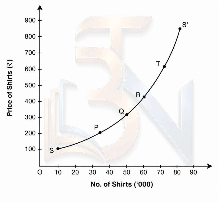
Fig 3. Supply Curve of Shirts
As shown in Figure 3, a supply curve has a positive slope. The positive slope of the supply curve is caused by seller’s desire to make larger profit and, more importantly, by the rise in cost of production. In fact, when price of a commodity increases, its suppliers tend to supply more and more. To supply more and more, they need to produce more and more. When they increase production, cost of production increases due to the law of diminishing returns. In fact, supply curve is derived from the marginal cost curve.
Shift in the Supply Curve
We have shown above that a change in the price of a commodity causes a change in its quantity supplied along a given supply curve. Although price of a commodity is the most important determinant of its supply, it is not the only determinant. Several other factors influence the supply of a commodity. Given the supply curve of a commodity, when there is a change in its other determinants, the supply curve shifts rightward or leftward depending on the effect of such changes. Let us now explain how other determinants of supply cause shift in the supply curve.
Change in input prices: Input prices include the price of labour, raw materials, overheads, etc. Input prices determine the cost of production. When input prices decrease, the use of inputs increases. As a result, product supply increases and the supply curve SS shifts to the right to SS”, as shown in Figure 4. Similarly, when input prices increase, product supply curve shifts leftward from SS to SS’.
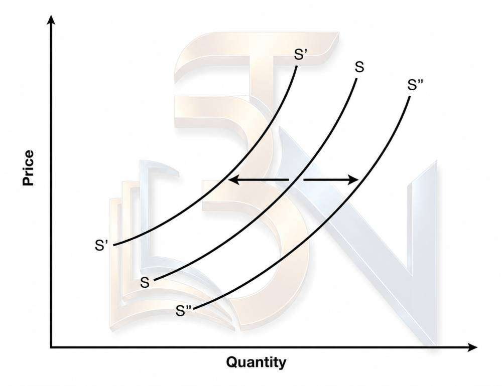
Fig. Shift in the Supply Curve
Technological progress: Technological progress reduces cost of production or increases labour productivity or does both. Technological progress that reduces cost of production or increases efficiency causes increase in product supply. For instance, introduction of high-yielding variety of paddy and new techniques of cultivation increased per-acre yield of rice in India in the 1970s. Such changes make the supply curve shift to the right.
Product diversification and cost reduction: In production of many commodities, it is possible to produce some other goods which require a similar technology. For example, a refrigerator company can also produce ACs; Tatas famous for truck production can also produce Nano and other types of cars; Maruti Udyog can produce trucks and so on. Product diversification may cause reduction in the production cost of the main product. This may lead to the rise in the supply of the main product due to capacity utilization for profit maximization.
Nature and size of the industry: The supply of a commodity depends also on whether an industry is monopolized or competitive. Under monopoly, supply of a product is shorter than it is in a competitive market. When a monopolized industry is made competitive, the total supply increases. Besides, if size of an industry increases due to new firms joining the industry, the total supply increases and supply curve shifts rightward.
Government policy: When government imposes restrictions on production, e.g., import quota on inputs, rationing of or quota imposed on input supply, etc., production tends to fall. Such restrictions make supply curve shift leftward.
Non-economic factors: The factors like labour strikes and lock-outs, war, droughts, floods, communal riots, epidemics, etc. also affect adversely the supply of commodities, making supply curve shift leftward.
Supply Function:
A supply function is a mathematical statement which states the relationship between the quantity supplied of a commodity and its determinants. The short-run market supply function is based on the law of supply. The law of supply states the nature of relationship between the price and the quantity supplied, i.e., supply increases with the increase in price. A supply function that specifies the relationship between the price and supply of a product is expressed as:
\( Q_x = dP_x \) ~ (2.6)
where:
\((Q_x)\) denotes the quantity supplied of commodity X.
\((P_x)\) denotes its price.
(d) gives the measure of relationship between \((Q_x)\) and \((P_x)\).
Once the relationship between \((Q_x)\) and \((P_x)\) is measured in numerical terms, i.e., the numerical value of ‘d’ is known, then the supply function can be expressed numerically. For example, suppose (d = 10), then the factual supply function can be expressed as:
\( Q_x = 10P_x \)
(2.7)
Given the supply function (2.7), a supply schedule can be obtained by substituting numerical values for \((P_x)\). For example:
If \((P_x = 2)\), then:
\( Q_x = 20 \)
If \((P_x = 5)\), then:
\( Q_x = 50 \)
By plotting the supply schedule, a supply curve can be obtained.
Consumer’s Equilibrium
Meaning:
Consumer’s equilibrium is a situation when he spends his given income on the purchase of one or more commodities in such a way that he gets maximum satisfaction and has no urge to change this level of consumption, given the prices of commodities.
Definition:
The state at which a consumer derives maximum utility from the consumption of one or more goods and services given his/her level of income is called Consumer’s Equilibrium. At that level of balance between total utility and income, the marginal utility of a product is equal to its one unit price.
Concept of Consumer’s Equilibrium:
Consumers derive utility from each commodity they consume. This utility is dependent on the price of a product. The point at which the marginal utility (MU) of a product equals its price (P) is where consumer satisfaction maximizes. It is expressed as MU = P. If the marginal utility of a product is higher than the price a consumer would continue to purchase additional units and vice versa until MU equals the fixed price level.
Importance of Consumer’s Equilibrium:
It allows a consumer to maximize his/her utility from the consumption of one or more commodities.
It helps arrange the combination of two or more products based on consumer taste and preference for maximum utility.
There are two main approaches to study consumer’s equilibrium. They are as follows:
Cardinal utility approach (or Marshall’s utility analysis)
Ordinal utility approach (or indifference curve analysis)
Law of Diminishing Marginal Utility and Equi Marginal Utility
The law of diminishing MU is the fundamental law on which is based the cardinal utility analysis of the consumer behaviour. This law states that as the quantity consumed of a commodity increases per unit of time, the utility derived by the consumer from the successive units goes on decreasing, provided the consumption of all other goods remains constant. This law is founded on the basis of some basic facts of life:
(i) the utility derived from a commodity depends on the intensity or urgency of the need for that commodity, and
(ii) as more and more quantities of a commodity is consumed, the need gets satisfied and therefore the intensity of need decreases.
For these reasons, the utility derived from the marginal unit goes on diminishing. For example, suppose you are very hungry and you are offered sandwiches to eat. The utility that you derive from the first piece of sandwich would be the maximum because intensity of your hunger is the highest. When you eat the second piece, you derive a lower satisfaction because intensity of your hunger is reduced. As you go on eating more and more sandwiches, the intensity of your hunger goes on decreasing and therefore the satisfaction which you derive from the successive units goes on decreasing.
If you continue to eat sandwiches, a point is reached when your hunger is fully satisfied and therefore the last piece of sandwich gives you zero utility. Eating sandwiches any more will give you a negative utility in the form of discomfort or stomachache. This relationship between quantity consumed and utility derived from each successive unit consumed is called the law of diminishing MU.
Numerical Example:
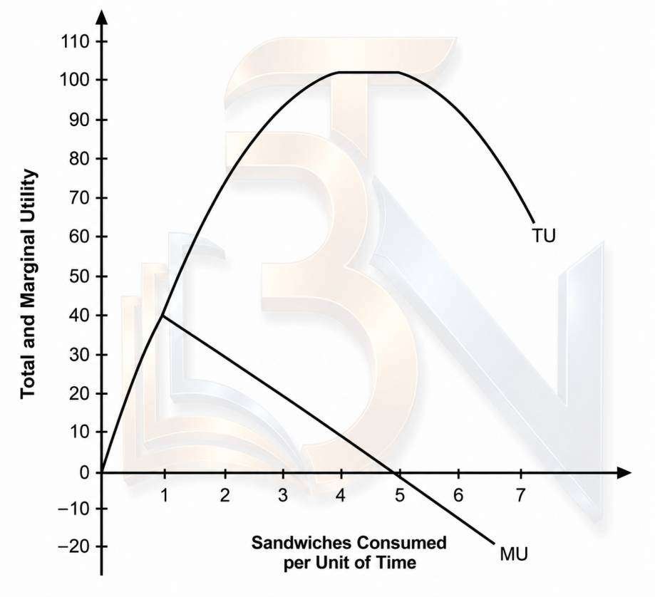
Table 5 presents a numerical illustration of the law of diminishing MU. As the table shows, TU increases with increase in consumption of sandwiches, but at a decreasing rate. It means that MU decreases with increase in consumption. This is shown in the last column of the table.
It can also be seen in the table that the TU reaches its maximum level at 100 at four sandwiches consumed. The consumption of the fifth sandwich gives no utility, i.e., its MU = 0.
\( MU = 0 \)
Consumption of the sixth sandwich yields a negative utility of 10 and the TU declines to 90.
Table 5: Total and Marginal Utility
| Sandwiches | Total Utility | Marginal Utility = \((TU_n – TU_{n-1})\) |
|---|---|---|
| 1 | 40 | (40 – 0 = 40) |
| 2 | 70 | (70 – 40 = 30) |
| 3 | 90 | (90 – 70 = 20) |
| 4 | 100 | (100 – 90 = 10) |
| 5 | 100 | (100 – 100 = 00) |
| 6 | 90 | (90 – 100 = -10) |
Graphical Illustration:
The law of diminishing MU is graphically illustrated in Figure 5. The TU and MU curves have been obtained by plotting the data given in Table 5. The TU curve is rising till the fourth sandwich is consumed. Note that the TU curve is rising but at a diminishing rate. It shows decrease in the MU, i.e., the utility added to the total.
The diminishing MU has been shown by the MU curve. Beyond five sandwiches consumed, the MU turns negative. It means that additional consumption of sandwiches yields disutility in the form of discomfort.
The law of diminishing MU is graphically illustrated in Figure 5. The TU and MU curves have been obtained by plotting the data given in Table 5. The TU curve is rising till the fourth sandwich is consumed. Note that the TU curve is rising but at a diminishing rate. It shows decrease in the MU, i.e., the utility added to the total.
The diminishing MU has been shown by the MU curve. Beyond five sandwiches consumed, the MU turns negative. It means that additional consumption of sandwiches yields disutility in the form of discomfort.
Assumptions:
The law of diminishing MU holds only under certain given conditions. These conditions are often referred to as the assumptions of the law.
First, the unit of the consumer goods must be standard, e.g., a cup of tea, a bottle of cold drink, a pair of shoes or a shirt and so on. If the units are excessively small or large, the law may not apply. For example, a sip of tea or a bite of sandwich may increase your desire for more tea or sandwich. It means that MU increases.
Secondly, consumer’s taste and preference remains unchanged during the period of consumption. If taste and preference change during the period of consumption, the law may not apply.
Thirdly, there must be continuity in consumption and where break in continuity is necessary, it must be appropriately short.
Fourthly, the mental condition of the consumer remains normal during the period of consumption. For, if a person is eating and also drinking alcohol the utility pattern will not be certain.
Given these conditions, the law of diminishing MU holds universally. In some cases, e.g., accumulation of money, collection of hobby items like stamps, old coins, rare paintings and books, and melodious songs, etc., MU may initially increase rather than decrease, but it does decrease eventually. That is, the law of MU generally operates universally.
Consumer’s Equilibrium: Cardinal Utility Approach
A consumer attains his equilibrium when he maximizes his TU given his income, consumption expenditure and prices of commodities he consumes. Analysing consumer’s equilibrium requires answering the question ‘how does a consumer allocate his money income to the various goods and services he consumes to arrive at his equilibrium?’ In this section, we explain how a consumer attains his equilibrium by applying the cardinal utility approach, under:
(i) the single commodity case, and
(ii) the multiple commodity case.
The cardinal utility approach, or what is also called as the Marshallian approach to consumer’s equilibrium, is based on the following assumptions.
Assumptions:
Rationality: It is assumed that the consumer is a rational being in the sense that he satisfies his wants in order of their merit and the necessity. It means that he buys first a commodity which yields the highest utility and he buys last a commodity which gives the least utility.
Limited Money Income: The consumer has a limited money income to spend on the goods and services he chooses to consume.
Maximization of Satisfaction: Every rational consumer intends to maximize his satisfaction from his given money income. That is, he chooses the commodities and spends his income on each of the commodity in such a way that his TU is maximized.
Utility is Cardinally Measurable: The cardinalists assume that utility is cardinally measurable, i.e., it can be measured in absolute terms and in cardinal numbers.
Diminishing MU: The consumption is subject to the law of diminishing marginal utility. That is, the utility derived from successive units of a commodity consumed decreases as a consumer consumes more and more units of it.
Constant Utility of Money: The MU of money remains constant whatever the level of consumer’s income and each unit of money has utility equal to one.
Utility is Additive: Cardinalists maintain that utility derived from different goods can be added up. The additivity of the utility can be expressed through a utility function. Suppose that the basket of goods and services consumed by a consumer contains (n) items, and their quantities may be expressed as \((x_1, x_2, x_3, \ldots, x_n)\). The utility function of the consumer may be expressed as:
$$U = f(x_1, x_2, x_3, \ldots, x_n)$$
Given the utility function, the TU obtained from (n) items may be expressed as:
$$U_n = U_1(x_1) + U_2(x_2) + U_3(x_3) + \ldots + U_n(x_n)$$
Single Commodity Case:
Having noted the assumptions of cardinal utility approach, we turn to analyse consumer’s equilibrium. As a general rule, a utility maximizing consumer consuming several commodities reaches his equilibrium when he maximizes his TU. However, for the sake of simplicity, we illustrate first consumer’s equilibrium with a simple one-commodity case.
Suppose that a consumer with a given money income consumes only one commodity, X. Since both his money income and commodity X have utility for him, he can either spend his money income on commodity X or retain it with himself. If he has total money and no commodity X, the MU of money will be lower than that of commodity X because:
$$MU_m = 1$$
But MU of commodity is supposed to be greater than 1. So long as \((MU_x)\) is greater than \((MU_m)\), TU can be increased by exchanging money for the commodity. Therefore, a utility maximizing consumer exchanges his money income for the commodity as long as:
$$MU_x > MU_m$$
As assumed earlier, MU of commodity X is subject to the law of diminishing returns (assumption 5), whereas MU of money income remains constant (assumption 6). Therefore, a utility maximizing consumer will exchange his money income for commodity X as long as:
$$MU_x > MU_m$$
The consumer reaches his equilibrium at the level of consumption at which:
$$MU_x = MU_m$$
In reality, however, the price of most goods is more than Re 1. In that case, the consumer’s equilibrium can be expressed as:
$$MU_x = P_x(MU_m)$$
where:
$$MU_m = 1$$
It implies that the consumer reaches equilibrium where:
$$\frac{MU_x}{P_x(MU_m)} = 1$$ ~ (2.8)
$$\frac{MU_x}{P_x(MU_m)} = 1$$ ~ (2.9)
Consumer’s equilibrium in a single commodity case is graphically illustrated in Figure 6. The horizontal line \((P_x(MU_m))\) shows the constant utility of money weighted by \((P_x)\) (the price of commodity X) and \((MU_x)\) curve represents the diminishing MU of commodity X. The \((P_x(MU_m))\) line and \((MU_x)\) curve intersect at point E, where:
$$MU_x = P_x(MU_m)$$
Therefore, consumer is in equilibrium at point E.
At any point above E,
$$MU_x > P_x(MU_m)$$
Therefore, if a consumer exchanges his money income for commodity X, he increases his satisfaction per unit of commodity.
At any point below E,
$$MU_x < P_x(MU_m)$$
the consumer can therefore increase his satisfaction by reducing his consumption of commodity X. That is, at any point other than E, the consumer gets satisfaction less than maximum. Therefore, point E is the point of consumer’s equilibrium.
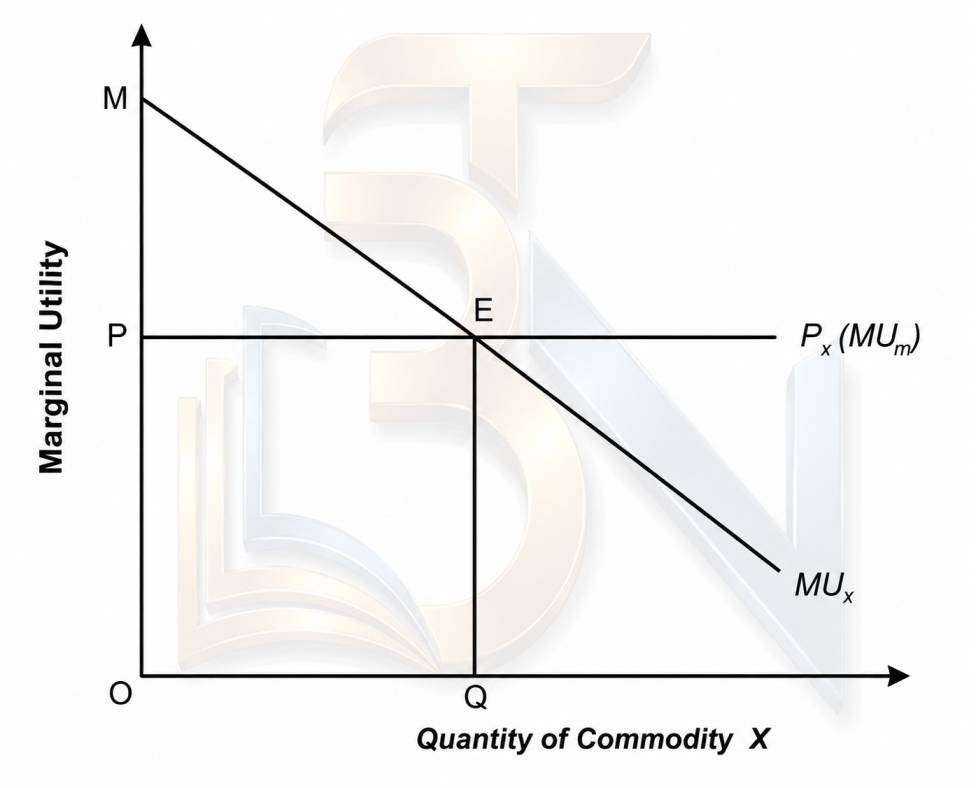
Fig 6. Consumer’s Equilibrium: One Commodity Case
The theoretical fact that the consumer is in equilibrium at point E can be proved by the data shown in Figure 6. As the figure reveals, the TU that the consumer derives by consuming OQ units of X equals the area OMEQ. The total money that consumer pays for OQ units equals:
$$OP \times OQ = OPEQ$$
This is the total utility of money paid for consuming OQ units.
When the total utility paid (OPEQ) is subtracted from the total utility gained (OMEQ), it gives the net utility gained. That is:
$$OMEQ – OPEQ = MPE$$
= net utility gain. The net utility gained (MPE) is maximum.
It can be checked that any consumption less than or more than OQ units will reduce the area MPE. So the consumer maximizes his utility at point E where:
$$MU_x = MU_m$$
The Multiple Commodity Case:
We have explained above the determination of consumer’s equilibrium in a single commodity case. In reality, however, a consumer consumes a large number of goods. Let us now see how a consumer consuming a large number of goods and services attains his equilibrium.
We know that the MU schedules of various commodities may not be the same. Some commodities yield higher utility and some lower. The MU of some goods decreases at a higher rate and of some at lower rate. A rational and utility maximizing consumer consumes commodities in the order of their utilities. He picks up the commodity which yields the highest utility and next he picks up the commodity which yields the second highest utility and so on. The consumer switches his expenditure from one commodity to another in accordance with their MU. He continues to switch his expenditure from one commodity to the other until he reaches a stage where MU of each commodity per unit of money expenditure is the same. This is called the law of equi-marginal utility.
The Law of Equi-Marginal Utility: Let us now present the law of equi-MU in a simple two-commodity case. Let us suppose that a consumer consumes only two commodities X and Y, and their prices are given as \(P_x\) and \(P_y\) respectively. Following the equilibrium rule of single commodity case, the consumer distributes his expenditure between commodities X and Y in such a way that:
$$MU_x = P_x(MU_m)$$
$$MU_y = P_y(MU_m)$$
or alternatively, consumer is in equilibrium where:
$$\frac{MU_x}{P_x(MU_m)} = 1$$ ~ (2.10)
$$\frac{MU_y}{P_y(MU_m)} = 1$$ ~ (2.11)
Equations (2.10) and (2.11) may be combined to express consumer’s equilibrium condition under two-commodity case as follows:
$$\frac{MU_x}{P_x(MU_m)} = 1 = \frac{MU_y}{P_y(MU_m)}$$ ~ (2.12)
Since, by assumption 5, MU of each unit of money remains constant, Eq. (2.12) may be rewritten as:
$$\frac{MU_x}{MU_y} = \frac{P_x}{P_y}$$ ~ (2.13)
or
$$\frac{MU_x}{P_x} = \frac{MU_y}{P_y}$$ ~ (2.14)
Equation (2.14) gives the utility maximization rule that the consumer reaches his equilibrium when the MU derived from each unit of money spent on the two commodities X and Y is the same.
The two-commodity case provides the basis for generalizing the consumer’s equilibrium by the cardinal utility approach in a multi-commodity case. In fact, a consumer consumes a large number of goods and services with his given income and at different prices. Supposing a consumer consumes A to Z goods and services, his equilibrium condition may be expressed as follows:
$$\frac{MU_A}{P_A} = \frac{MU_B}{P_B} = \frac{MU_C}{P_C} = \cdots = \frac{MU_Z}{P_Z}$$ ~ (2.15)
Thus, according to the law of equi-marginal utility, a utility maximizing consumer consuming several goods and services intends to equalize the MU of each unit of his money spent on various goods and services.
Consumer Surplus
The consumers’ willingness to pay for a commodity depends on the utility they expect to derive from the commodity. The price which a consumer is willing to pay may not match with the market price of the commodity. It may be greater or less than the market price. If market price is less than what the consumer is willing to pay, then he saves some money. In economics terminology, this saving is called consumer surplus.
The concept of consumer’s surplus is believed to have been originated by a French engineer, Arsene Julis Dupuit, in 1844, in his effort to measure social benefit of such collective goods as roads, canals and bridges. In his opinion, the value of the benefit of such collective goods was greater than the price actually charged because most people would be willing to pay a higher price than they actually paid. The concept was later refined by Marshall who also provided a measure of consumer’s surplus. His premise of measuring consumer’s surplus was, however, rejected by the ordinalists, especially J.R. Hicks, who attempted to provide a different method of measuring consumer’s surplus through their indifference curve technique.
There are various methods of measuring consumer’s surplus and their merits and demerits. In this section, you will learn about the Marshallian concept and measure of consumer surplus and its drawbacks.
Marshallian Concept of Consumer Surplus
Although the concept of consumer surplus was originated by Dupuit as early as 1844, it remained an immeasurable concept until Marshall suggested, as late as 1920, a method of measuring consumer’s surplus in money terms. Marshall defined consumer’s surplus as “the excess of the price which [a consumer] would be willing to pay rather than go without the thing, over that which he actually does pay.” According to the Marshallian theory of demand, what a consumer is willing to pay for one unit of a commodity measures the money value of his expected utility and what he actually pays gives the measure of the monetary cost of the expected utility. According to Marshall, the difference between the two values is the ‘consumer surplus’. For example, if you are prepared to pay ₹500 for a ticket to watch a cricket match and you pay only ₹200, the actual price of the ticket, you have a consumer surplus of ₹300.
The concept of consumer’s surplus can be expressed also in terms of utility (or satisfaction). Recall that Marshall assumed marginal utility (MU) of money to remain constant. Under this condition, what a consumer is willing to pay for a commodity indicates the utility that he expects to derive from the commodity and what he actually pays gives the measure of the loss of utility (of money). The difference between the utility gained and the utility lost in acquiring the commodity is the consumer’s ‘surplus satisfaction’ which Marshall called ‘consumer’s surplus’.
Measurement of Consumer Surplus:
Having defined the concept of consumer surplus, Marshall provided a systematic method of measuring the consumer surplus, on the basis of certain assumptions.
Assumptions: The Marshall’s method of measuring consumer’s surplus is based on the following assumptions.
First, it is assumed that the market price is given so that neither the sellers nor the buyers can affect the price. The consumer’s surplus will not exist if there is a monopolist and he adopts first degree price discrimination in his pricing policy.
Secondly, the utility is cardinally measurable and MU of consumer’s money income remains constant throughout.
Thirdly, the utility of each commodity is absolute and is independent of other goods and services consumed by the consumer.
Fourthly, there is no close substitute for the commodity in question. For, if close substitutes are available, there may not be any difference between ‘what the consumer would be willing to pay’ and ‘what he actually pays’ for the commodity in question.
The Marshallian concept of consumer’s surplus and its measurement are graphically illustrated in Figure 7. Suppose the consumer’s demand curve for a commodity X is given by the demand curve MN. The curve MN also indicates the utility derived from each successive unit of a commodity and the price that the consumer is willing to pay at different levels of his purchases. Suppose that the market price, i.e., the price which a consumer actually pays, is given by OP. At price OP, the consumer buys OQ units. The total utility derived by the consumer from OQ units is shown by the area OMBQ, for which the consumer pays:
$$OPBQ = OQ \times OP$$
Thus, in the Marshallian sense, total consumer surplus equals:
$$OMBQ – OPBQ = MPB$$
That is, the shaded area MPB represents the consumer’s surplus in the Marshallian sense when the consumer buys OQ units of a commodity X.
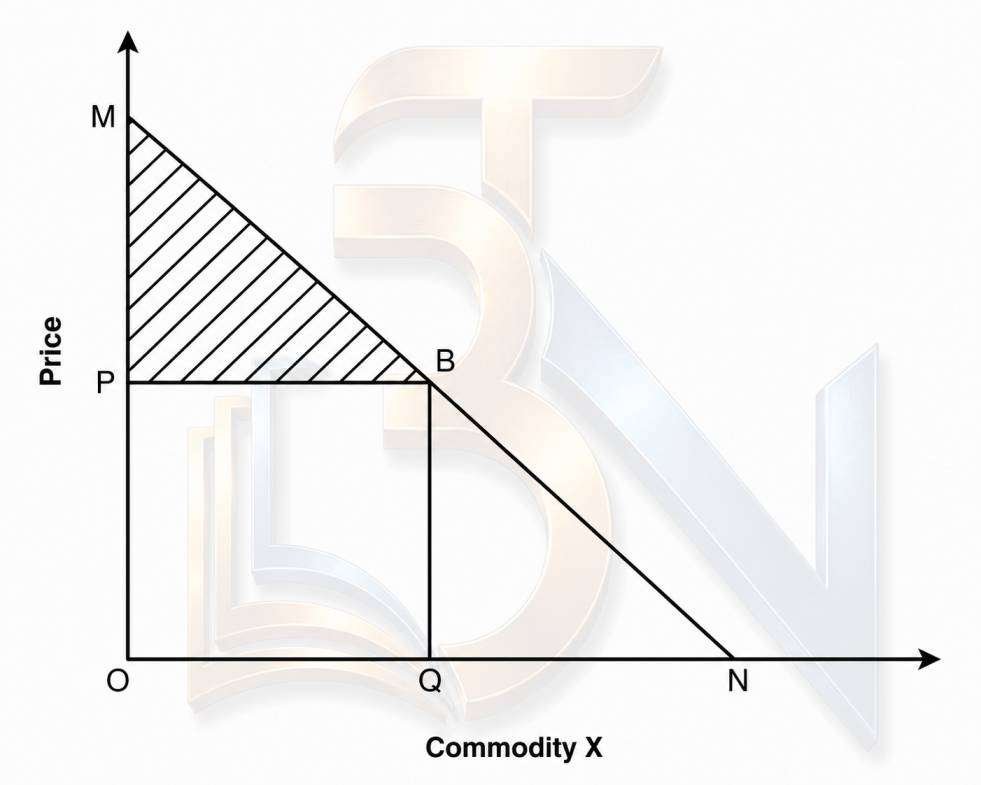
Critical Appraisal
The Marshallian concept and measurement of consumer’s surplus have been criticized on many grounds, though the criticisms are equally questionable. The criticism of Marshallian concept of consumer surplus and its validity are discussed below.
First, economists have pointed out difficulties in measuring the consumer’s surplus as defined by Marshall and represented by ‘a triangle’. A triangle cannot be formed because consumer’s willingness to pay for zero unit is unknown. So demand curve cannot be extend to price axis. However, Mark Blaug rejects this criticism. In the words of Mark Blaug, ‘It is sometimes objected that demand curves are usually asymptotic to the price axis. If the individual’s offer for the first unit is not defined so that the demand curve does not touch the Y-axis, the integral under the demand curve is infinite. But this objection is easily overcome by measuring consumer’s surplus from some selected value of \(q_x > 0\).’
Secondly, a ‘more fatal objection’ to Marshall’s method of measuring consumer’s surplus as ‘the triangle’ under the demand curve is that real income does not remain constant along the demand curve even for ‘unimportant’ commodities. As the price falls along the demand curve (as shown in Figure 7), real income makes the estimate of consumer’s surplus as ambiguous one. This criticism too does not hold because increase in demand due to decrease in price is caused also by its income effects.
Thirdly, it is generally alleged that Marshallian assumptions on which the measurement of consumer’s surplus is based are unrealistic. It is argued that MU of money does not remain constant; cardinal measurement of utility is not possible; utilities of various goods consumed by a consumer are not independent of each other; most goods have their substitutes—close or remote, and so on. Therefore, it is alleged that the Marshallian concept of consumer’s surplus is imaginary and hypothetical. However, this criticism too does not hold in literal sense. Although utility may not be measurable cardinally or ordinally, consumers do have a mental perception of the usefulness of a commodity and, accordingly, they have a willingness to pay an amount for a commodity they need. It is not hypothetical.
Fourthly, in the ultimate analysis of the consumer’s purchases of various goods and services, consumer’s surplus is reduced to zero. For, a consumer’s willingness to pay (i.e., ‘potential price’) cannot exceed his income, i.e., what he actually pays out. It means that, when all purchases have been made, the consumers willingness to pay (which equals his income) equals what he actually pays (i.e., his income). This criticism is more hypothetical than the concept of consumer surplus as claimed by some economists.
Fifthly, the concept of consumer’s surplus cannot be convincingly applied to ‘essential’ and prestigious goods. For example, a hungry affluent person may be willing to pay thousands of rupees for a piece of bread whereas he may be required to pay only ten rupees. As such, his consumer’s surplus will be equal to 99,990 which seems ridiculous. In case of prestigious goods, e.g., rare paintings, diamonds, jewellery, etc., what a buyer is willing to pay, generally, equals what he actually pays. It means there is no consumer’s surplus. Thus, Marshallian concept of consumer surplus becomes illusory. However, these cases may be exceptions and exceptions prove the rule.
Although criticisms of Marshallian concept of consumer surplus are not strong enough to reject the concept, Samuelson considers this concept as of only ‘historical and doctrinal interest’ and suggests that ‘the economists had best dispense with it’. Hicks has, however, tried to rehabilitate the consumer’s surplus as, in his opinion, this concept is of great importance in the economics of welfare and also from pricing policy point of view.
Indifference Curve
The indifference curve is defined as the locus of points each point representing a different combination of two goods yielding the same utility or level of satisfaction. Since utility expected from the different combinations of the two goods is the same, a rational consumer is indifferent between any two combinations of goods when it comes to making a choice between them.
Such a situation arises because a consumer consumes a large number of goods and services and often finds that one commodity can be used as substitute for another. This gives the consumers an opportunity to substitute one commodity for another. In that case, they are able to form various combinations of two substitute goods that give them the same level of satisfaction. When a consumer is faced with such combinations of goods, he would be indifferent between the combinations. When such combinations are plotted graphically, it appears in the form of a curve. This curve is known as the indifference curve. Indifference curves are also called iso-utility or equal utility curves.
For example, let us suppose that a consumer forms five combinations a, b, c, d and e of two commodities, X and Y, as presented in Table 6. All these combinations yield the same level of satisfaction (U). The consumer is, therefore, indifferent to the choice between them. The five combinations of the two commodities X and Y may be called as an indifference schedule.
Table 6 shows five combinations of two goods, X and Y, which give the same utility. The last column of the table shows an unquantified utility (U) derived from each combination of X and Y. Utility (U) is unquantified because, under the ordinal utility approach, utility is not measurable quantitatively.
Table 6: Indifference Schedule of Commodities X and Y
| Combination | Commodity X | + | Commodity Y | Utility | ||
|---|---|---|---|---|---|---|
| a | = | 25 | + | 5 | = | (U) |
| b | = | 15 | + | 7 | = | (U) |
| c | = | 10 | + | 12 | = | (U) |
| d | = | 6 | + | 20 | = | (U) |
| e | = | 4 | + | 30 | = | (U) |
When the combinations a, b, c, d and e given in Table 6 are plotted and joined by a smooth curve (as shown in Figure 8), the resulting curve IC is known as the indifference curve.
On this curve, one can locate many other points showing many other combinations of X and Y, which yield the same level of satisfaction. Therefore, the consumer is indifferent to make choice between the points on the indifference curve. Therefore, the curve is called the ‘indifference curve’.
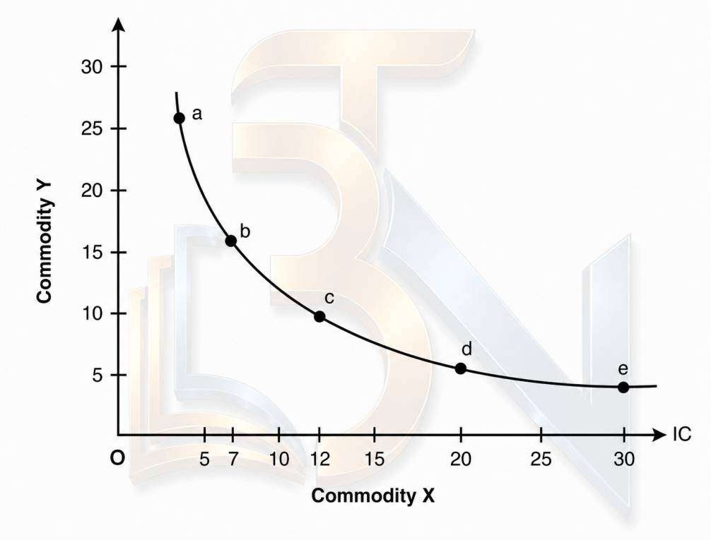
Fig 8. Indifference Curve
Indifference Map
Figure 8 presents a single indifference curve IC drawn on the basis of the indifference schedule given in Table 6. The consumer can similarly frame many other combinations of X and Y with less amounts of both the goods such that each combination yields the same level of satisfaction but less than the level of satisfaction indicated by the indifference curve IC in Figure 8.
Similarly, a consumer can concoct many other combinations with more of both the goods—each combination yielding the same satisfaction, but yielding a greater level of satisfaction than the smaller combination. Thus, another indifference curve can be drawn above the IC curve.
This exercise may be repeated as many times as one wants, each time generating a new indifference curve. A set of indifference curves constitute the indifference map, as shown in Figure 9.
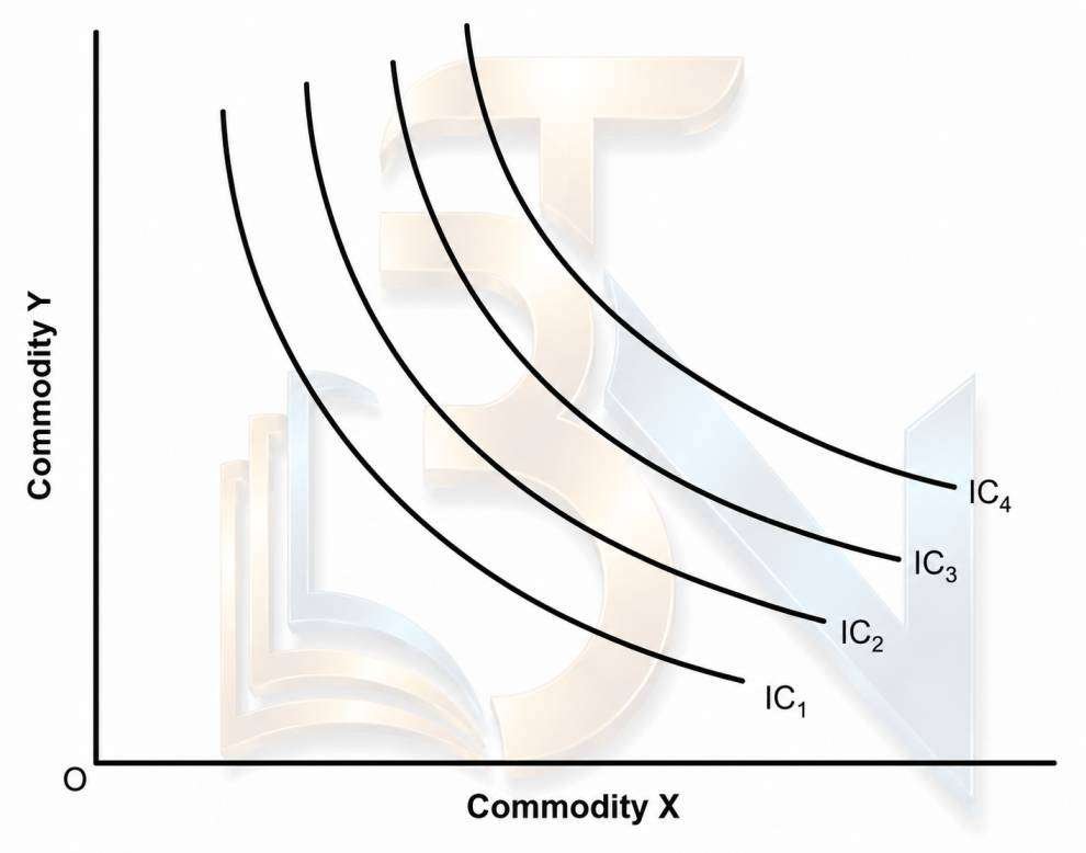
In fact, the area between the X and the Y axes is known as the indifference plane or the commodity space. This plane contains finite points and each point on the plane indicates a different combination of the goods X and Y. Intuitively, it is always possible to locate two or more points indicating different combinations of the goods X and Y yielding the same level of satisfaction.
It is thus possible to draw a number of indifference curves that neither intersect nor are tangent to one another, as shown in Figure 9. The set of indifference curves, IC1, IC2, IC3 and IC4, drawn in this manner constitute the indifference map.
In fact, an indifference map may contain any number of indifference curves ranked in the order of consumer’s preferences.
Characteristics of Indifference Curves
The indifference curve is a tool of analysis. As a tool of analysis, it has the following four basic properties:
Indifference curves slope downward to the right.
Indifference curves combining imperfect substitutes are convex to the origin.
Indifference curves do not intersect nor are they tangent.
An upper indifference curve implies a higher level of satisfaction than the lower ones.
Indifference curves slope downward to the right: In the words of Hicks, ‘So long as each commodity has a positive marginal utility, the indifference curve must slope downwards to the right’. The downward slope of an indifference curve implies that in a basket of two substitute goods, if the quantity of one commodity decreases, the quantity of the other commodity must increase if the consumer has to maintain the same level of satisfaction. If the quantity of the other commodity does not increase simultaneously, the basket of commodities decreases with the decrease in the quantity of one commodity. In that case, a smaller bundle of goods is bound to yield a lower level of satisfaction, which defies the logic of indifference curve.
Indifference curves are convex to the origin: Indifference curves for normal goods have not only a negative slope, but are also convex to the origin. The convexity of the indifference curves is caused by the following factors:
The two goods are imperfect substitutes for one another.
The diminishing MRS incase of imperfect substitutes.
Indifference curves neither intersect nor are tangent to one another: If two indifference curves intersect or are tangential to each other, it would imply two types of inconsistencies in indifference curve logistics:
Upper and lower indifference curves indicate the same level of satisfaction.
The bigger and smaller combinations of two goods yield the same level of satisfaction.
Such conditions are improbable if a consumer’s subjective valuation of utility of a commodity is greater than zero. Obviously, if two indifference curves intersect, it would mean a violation of the consistency or transitivity assumption for consumers’ preferences.
Let us now prove the point graphically. Suppose two indifference curves, IC1 and IC2, intersect at point A, as shown in Figure 10. Consider two other points—point B on the indifference curve IC1 and point C on the indifference curve IC2, both falling on a vertical line. Points A, B and C represent three different combinations of commodities X and Y. Let us call these combinations, respectively, as combination A, B and C. Note that combination A is common to both the indifference curves. Since points A and B fall on the same IC curve IC1, it means that, in terms of utility:
$$A = B$$
Similarly, since points A and C fall on the same indifference curve, IC2, it means that, in terms of utility:
$$A = C$$
Since A = B and A = C, it means that:
$$B = C$$
However, if combinations of goods at points B and C yield the same utility, it would mean that, in terms of utility:
$$ON\ of\ X + BN\ of\ Y = ON\ of\ X + CN\ of\ Y$$
Since ON of X is common to both the terms, it means that utility of BN of Y is equal to utility of CN of Y. However, as Figure 10 shows, BN > CN. Therefore, combinations at B and C cannot be equal in terms of utility in the subjective introspection of the consumer. The intersection of indifference curves, therefore, violates the transitivity rule, which is a logical necessity in indifference curve analysis.
$$BN > CN$$
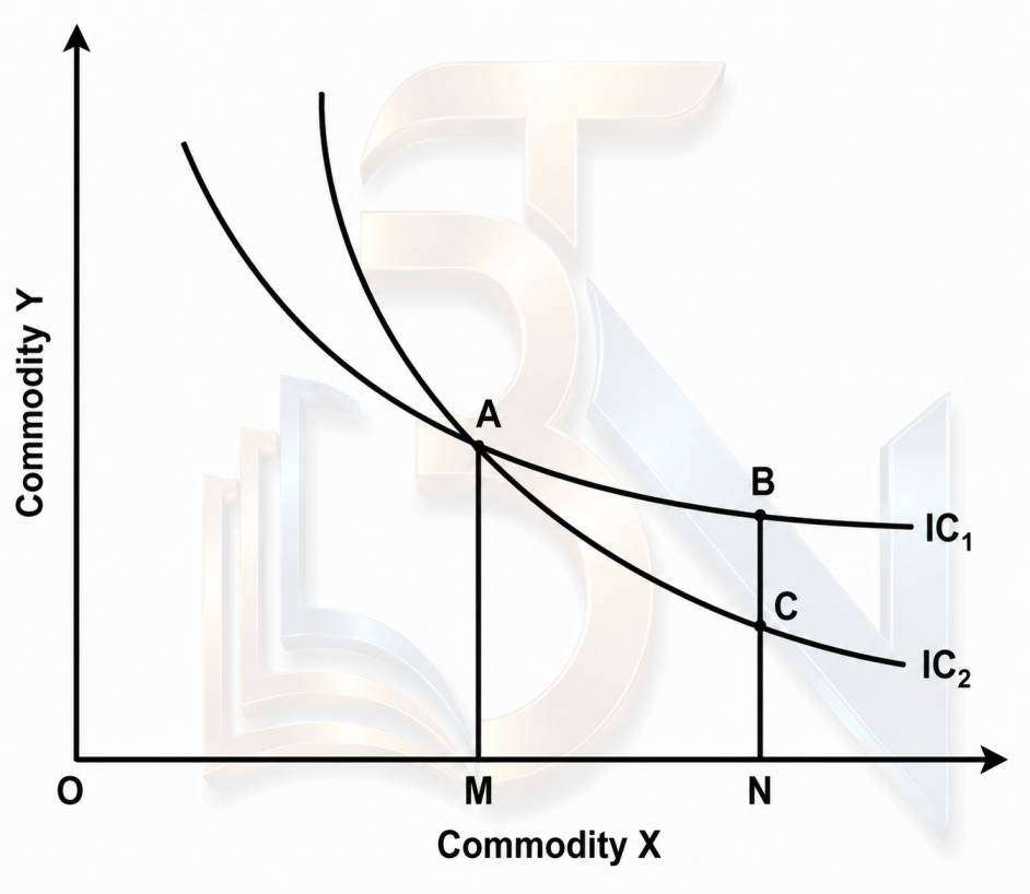
Fig. Intersecting Indifference Curves
Higher indifference curves represent a higher level of satisfaction than the lower ones: An indifference curve placed above and to the right of another represents a higher level of satisfaction than the lower one. The reason is that an upper indifference curve contains all along its length a larger quantity of one or both the goods than the lower one. In reality, a larger quantity of a commodity is supposed to yield a greater satisfaction than a smaller quantity of the same commodity, provided its:
$$MU > 0$$
For example, consider the indifference curves IC1 and IC2 in Figure 11. The vertical movement from point a on the lower indifference curve, IC1, to point b on the upper indifference curve, IC2, means an increase in the quantity of Y by ab, the quantity of X remaining the same (OX). Similarly, a horizontal movement from point a to point d means a greater quantity of commodity X, the quantity of Y remaining the same (OY). A diagonal movement from point a to point c means larger quantities of both X and Y. Unless the utility of additional quantities of X and Y are equal to zero, these additional quantities will yield additional utility. Therefore, the level of satisfaction indicated by the upper indifference curve IC2 would always be greater than that indicated by the lower indifference curve IC1.
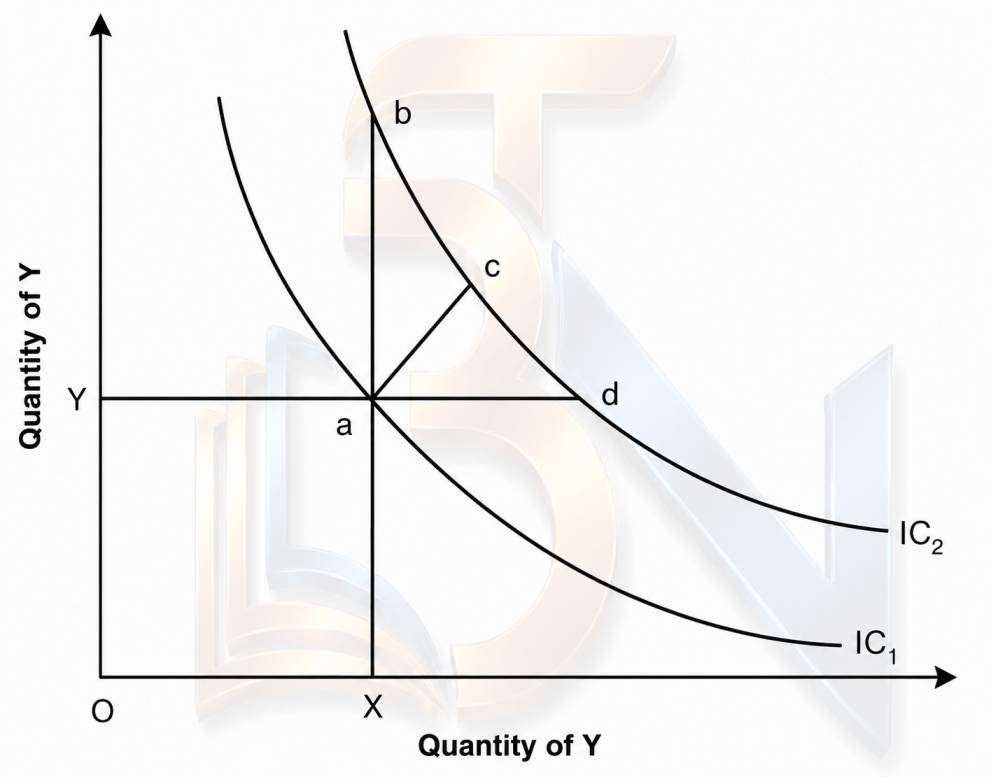
Consumer’s Equilibrium: Ordinal Utility Approach
Marginal Rate of Substitution:
When a consumer makes different combination of two goods, yielding the same level of satisfaction, he substitutes one good for another. The rate at which he substitutes one good for the other is called the Marginal Rate of Substitution, (MRS). One of the basic postulates of indifference curve analysis is that (MRS) diminishes. The axiomatic assumption of ordinal utility theory is analogous to the assumption of Diminishing Marginal Utility in cardinal utility theory.
The postulate of diminishing marginal rate of substitution states an observed behavioural rule that when a consumer substitutes one commodity (say X) for another (say Y), the Marginal Rate of Substitution (MRS) decreases as the stock of X increases and that of Y decreases.
Conceptually, the MRS is the rate at which one commodity can be substituted for another, the level of satisfaction remaining the same. The MRS between two commodities, X and Y, can also be defined as the number of units of X which are required to replace one unit of Y (or number of units of Y that are required to replace one unit of X), in the combination of the two goods so that the total utility remains the same. It implies that the utility of units of X (or Y) given up is equal to the utility of additional units of Y (or X) added to the basket.
The negative slope of the indifference curve implies that two commodities are not perfect substitutes for each other. In case they are perfect substitutes, the indifference curve will be a straight line with a negative slope. Since, goods are not perfect substitutes for each other, the subjective value attached to the additional quantity (i.e., MU) of a commodity decreases fast in relation to the other commodity whose total quantity is decreasing.
Budget Line, Budget Constraint and Budget Line:
A utility maximising consumer would like to reach the highest possible indifference curve on his indifference map. However, the consumer is assumed to have a limited income. Limited income sets a limit to which a consumer can maximise his utility. The limitedness of income acts as a constraint. This is known as budgetary constraint. The assuming a two-commodity model, budgetary constraint may be expressed as:
$$P_x \cdot Q_x + P_y \cdot Q_y = M$$
Where \(P_x\) and \(P_y\) are respective prices of X and Y, and \(Q_x\) and \(Q_y\) are their respective quantities; (M) is consumer’s money income. Equation (2.16) states that a consumer, given his income and prices of X and Y in the market, can buy only limited quantities of the two goods – X and Y. The maximum \(Q_x\) and \(Q_y\) can be obtained from Eq. (2.16), as follows.
Equation (2.17a):
$$Q_y = \frac{M}{P_y} – \frac{P_x}{P_y} \times Q_x$$
Equation (2.17b):
$$Q_x = \frac{M}{P_x} – \frac{P_y}{P_x} \times Q_y$$
Equations (2.17a) and (2.17b) are budget equations. Given the budget equations if values of (M), \(P_x\) and \(P_y\) are known, then the values of \(Q_y\) and \(Q_x\) can be easily calculated. For example, if \(Q_x = 0\) then \(Q_y = \frac{M}{P_y}\) and if \(Q_y = 0\) then \(Q_x = \frac{M}{P_x}\). Similarly, \(Q_x\) and \(Q_y\) may be alternatively assigned a positive numerical value and the corresponding values of \(Q_x\) and \(Q_y\) calculated. When the values of \(Q_x\) and \(Q_y\) are plotted on X and Y axis, it gives a line with a negative slope, which is called budget line or price line, as shows in Fig. 12.
If \(Q_x = 0\):
$$Q_y = \frac{M}{P_y}$$
If \(Q_y = 0\):
$$Q_x = \frac{M}{P_x}$$
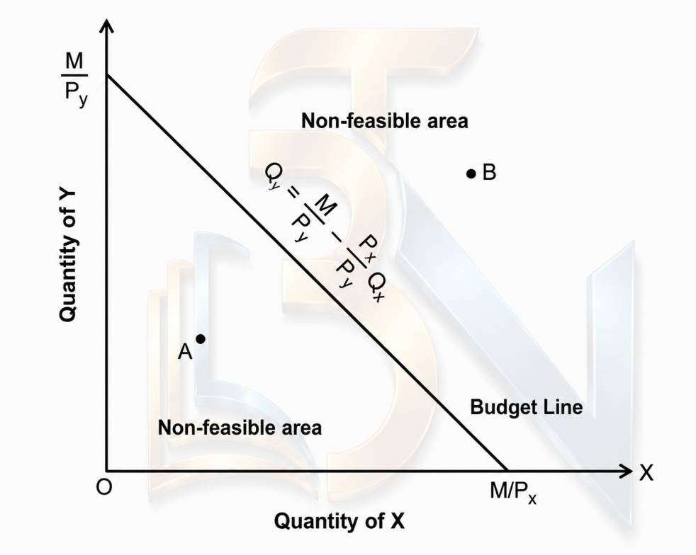
An easier method of deriving the budget line is to be find the point \(M/P_y\)
on Y-axis (assuming
$$Q_x = O$$ and point $$M/P_x$$
on X-axis (assuming $$Q_y = O$$
By joining these points by a line, one can obtain the budget line as given by the budget equation in Fig. 12.
The budget line divides the commodity space into two parts which may be termed as:
(i) feasibility area
(ii) non-feasibility area
The area lying in the south-west of the budget line is feasibility area (Fig. 12). For, any combination of goods X and Y represented by a point within the area (e.g., point A) or on the boundary line (i.e., budget line) is a feasible combination, given
\(M\) , \(P_x\) and \(P_y\)
The area in the north-east of the budget line is non-feasibility area because any point falling in this area, e.g., point B, is unattainable (given
\(M\) , \(P_x\) and \(P_y\)
Let us now look at the factors that shift budget line, and the slope of the budget line.
(a) Shifts in Budget Line:
The budget line changes its position following the change in consumer’s income and prices of the commodities. If consumer’s income increases, prices of X and Y remaining the same, budget line shifts upwards remaining parallel to the original budget line. Likewise, income remaining the same, if prices change, the budget line changes its position.
(b) Slope of the Budget Line:
The slope of the budget line is of great importance in determining consumer’s equilibrium. The slope of the budget line (AB) in Fig. 13 is given by the following ratios.
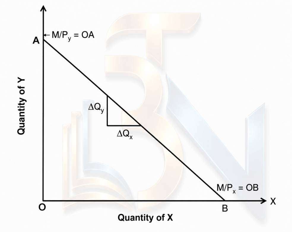
Since OA = M/Py and OB = M/Px (Fig. 13) the slope of the budget line may be rewritten as
$$\frac{OA}{OB}\;=\;\frac{M/P_y}{M/P_x}\;=\;\frac{P_y}{P_x}$$
As Eq. (2.18) shows, the slope of the budget line equals the price ratio (Py / Px ).
Consumer’s Equilibrium:
As noted above, consumer’s equilibrium attains when he maximises total utility, given his income and market prices of goods and services he consumes. Under indifference curve analysis of consumer behaviour, necessary condition for total utility to be maximum is that MRS must be equal to the ratio of commodity prices. Considering our earlier two-commodity models, the necessary (or the first order) condition may be expressed as:
\[ MRS_{xy}=\frac{MU_x}{MU_y}=\frac{P_x}{P_y} \]
This is a necessary condition but not sufficient condition of consumer’s equilibrium. Another condition, a second order or supplementary condition is that the necessary condition must be fulfilled at the highest possible indifference curve.
Consumer’s equilibrium is illustrated in Fig. 14. A hypothetical indifference map of the consumer is shown by indifference curves \(IC_1\), \(IC_2\) and \(IC_3\). The line AB is the hypothetical budget line. Both necessary and supplementary conditions of consumer’s equilibrium are fulfilled at point E, where indifference curve \(IC_2\) is tangent to the budget line, AB. Since both, the curve \(IC_2\) and the budget line, AB, pass through point E, therefore, at this point, the slopes of the indifference curve \(IC_2\) and the budget line (AB) are equal. The consumer is therefore in equilibrium at point E.
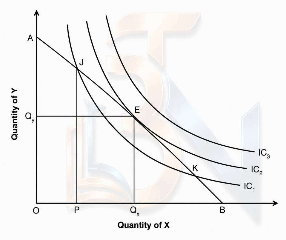
That the consumer is in equilibrium at point E can also be proved algebraically. We know that the slope of an indifference curve is given by:
\[ -\frac{\Delta Y}{\Delta X}=\frac{MU_x}{MU_y}=MRS_{y,x} \]
We know also that the slope of the budget line is given by Eq. (2.17) as:
\[ \frac{OA}{OM}=\frac{P_y}{P_x} \]
At point E:
\[ MRS_{y,x}=\frac{P_y}{P_x} \]
Therefore, the consumer is in equilibrium at point E.
The tangency of \(IC_2\) with the budget line indicates that \(IC_2\) is the highest possible indifference curve which the consumer can reach, given his budgetary constraint and the prices. At equilibrium point E, the consumer consumes \(OQ_x\) of X and \(OQ_y\) of Y, which yield him maximum satisfaction.
Although, the necessary condition is satisfied also on two other points, J and K, these points do not satisfy the supplementary or the second order condition of consumer’s equilibrium. Indifference curve \(IC_1\) is not the highest possible curve on which the necessary condition is fulfilled. Since, indifference curve \(IC_1\) lies below the curve \(IC_2\), at any point on \(IC_1\), the level of satisfaction is lower than the level of satisfaction indicated by \(IC_2\). So long as the utility maximising consumer has the opportunity to reach the curve \(IC_2\), he would not like to settle on a lower curve.
From the information contained in Fig. 14, it can be proved that the level of satisfaction at point E is greater than that on any point on \(IC_1\). Suppose that the consumer is at point J. If he moves to point M, he will be equally well-off because points J and M are on the same indifference curve. If he moves from point J to M, he will have to sacrifice JP of Y and take PM of X. But in the market, he can exchange JP of Y for PE of X. That is, he gets extra ME (PE − PM) of X. Since ME gives him extra utility, point E yields a utility higher than the point M. Therefore, point E is preferable to point M. The consumer will therefore have a tendency to move to point E from any point at the curve \(IC_1\), in order to reach the highest possible indifference curve, all other things (taste, preference, and prices of goods) remaining the same.
Another fact which is obvious from Fig. 2.14 is that, due to budget constraint, the consumer cannot move to an indifference curve placed above and to the right of \(IC_2\). For example, his income would be insufficient to buy any combination of two goods at the curve \(IC_3\). Note that \(IC_3\) falls beyond the budget line.
To conclude, a utility maximising consumer, given his income, taste and preferences and prices of goods, will attain his equilibrium when:
\[ MRS=\text{price ratio} \]
at the highest possible indifference curve.