
Introduction
The Theory of Production and Costs is one of the cornerstones of microeconomic analysis and focuses on how firms derived production function decisions in a way to maximize their profit and minimize costs. It deals with the study of inputs, especially in the form of labor and capital inputs that go into making, against related outputs of goods and services, and also the cost involved in producing those outputs.
The knowledge of such principles is very important for any business firm to optimize its production processes, efficiently allocate resource supplies, and define price strategies in competitive markets. These important concepts are the production and cost functions that define the input-output relationship and further quantify expenses incurred in the production of goods and services, respectively. With this background, economists and business managers can look into productiveness in production, efficient decisions about resource allocation, and strategy making toward profitability and sustainability.
Production Function
Production Function expresses a functional relationship between physical inputs and physical outputs of a firm at any particular time period. The output is thus a function of inputs.
Mathematically production function can be written as:
$$Q = f(L_1, L_2, C, O, T)$$
Where Q stands for the quantity of output and various input factors such as L₁ as land, L₂ as labour, C is capital, O is organization and T is technology.
Here output is the function of inputs. Hence output becomes the dependent variable and inputs are the independent variables.
Definition:
Michall R. Baye “the function which defines the maximum amount of output that can be produced with a given set of inputs.
As part of economics, theory of production and cost investigates how firms mix inputs to make outputs and how this process affects their costs. The course outline is as follows:
Isoquants
An isoquant is a curve representing the various combinations of two inputs that produce the same amount of output. An isoquant curve is also known as iso-product curve, equal-product curve, and production indifference curve.
A curve which shows the different combinations of the two inputs producing a given level of output.
| Combinations | Labour (units) | Capital (Units) | Output (quintals) |
|---|---|---|---|
| A | 1 | 10 | 50 |
| B | 2 | 7 | 50 |
| C | 3 | 4 | 50 |
| D | 4 | 4 | 50 |
| E | 5 | 1 | 50 |
Combination ‘A’ represent 1 unit of labour and 10 units of capital and produces ‘50’ quintals of a product. All other combinations in the table are assumed to yield the same given output of a product, say ‘50’ quintals, by employing any one of the alternative combinations of the two factors, labour and capital.
If we plot all these combinations on a paper and join them, we will get continues and smooth curve called Iso-product curve as shown below.
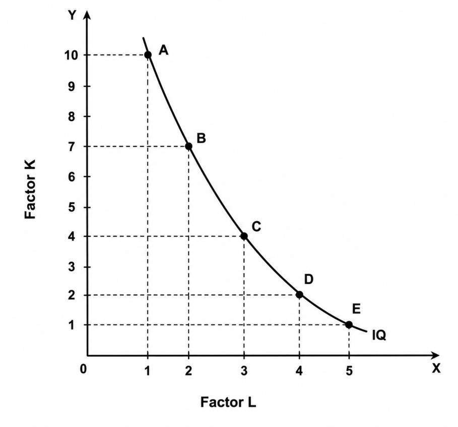
Labour is on the X-axis and capital is on the Y-axis. IQ is the ISO-Product curve which shows all the alternative combinations A, B, C, D, E which can produce 50 quintals of a product.
Features of Isoquant:
- Downward sloping: Isoquants are downward sloping curves because, if one input increases, the other one reduces. There is no question of increase in both the inputs to yield a given output. A degree of substitution is assumed between the factors of production.
- Convex to origin: Isoquants are convex to the origin. Because the input factors are not perfect substitutes. One important factor can be substituted by the other input factor in a “Diminishing marginal rate.”
- If the input factors were perfect substitutes, the isoquants be a falling straight line.Do not intersect– Two isoproducts do not intersect with each other.
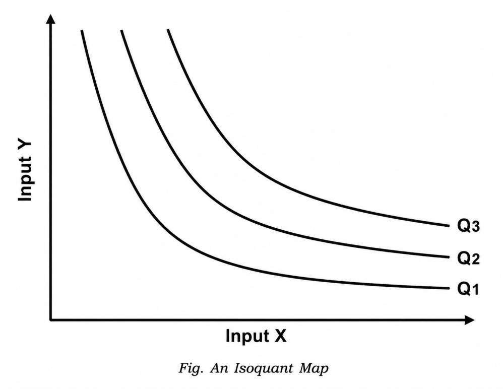
Do not touch axes- The isoquants touches neither X-axis nor Y-axis, as both inputs are required to produce a given product
Marginal Rate of Technical Substitution (MRTS)
Definition:
Prof. R.G.D. Alien and J.R. Hicks introduced the concept of MRS (marginal rate of substitution) in the theory of demand. The similar concept is used in the explanation of producers’ equilibrium and is named as marginal rate of technical substitution (MRTS).
Marginal rate of technical substitution (MRTS) is: “The rate at which one factor can be substituted for another while holding the level of output constant”. The slope of an isoquant shows the ability of a firm to replace one factor with another while holding the output constant.
For example, if 2 units of factor capital (K) can be replaced by 1 unit of labor (L), marginal rate of technical substitution (MRTS) will be thus:
$$MRTS_{LK}\;=\;\frac{\triangle K}{\triangle L}$$
| Combination | Capital (Rs. in lakh) | Labour | Marginal Rate of Technical Substitution (MRTS) |
|---|---|---|---|
| A | 1 | 20 | — |
| B | 2 | 15 | 5:1 |
| C | 3 | 11 | 4:1 |
| D | 4 | 8 | 3:1 |
| E | 5 | 6 | 2:1 |
| F | 6 | 5 | 1:1 |
It means that the marginal rate of technical substitution of factor labor for factor capital (K).(MRTSLK) is the number of units of factor capital (K) which can be substituted by one unit of factor labor (L) keeping the same level of output.
Isocosts
The cost curve that represents the combination of inputs that will cost the producer the same amount of money (or) each isocost denotes a particular level of total cost for a given level of production. If the level of production changes, the total cost changes and thus the isocost curve moves upwards, and vice versa.
Least Cost Factor Combination Of Inputs:
The firm can achieve maximum profits by choosing that combination of factors which will cost it the least. The choice is based on the prices of factors of production at a particular time. The firm can maximize its profits either by maximizing the level of output for a given cost or by minimizing the cost of producing a given output.
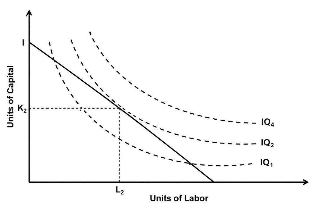
The least cost factor combination can be determined by imposing the isoquant map on isocost line.
The point of tangency between the isocost and an isoquant is an important but not a necessary condition for producer’s equilibrium.
The essential condition is that the slope of the isocost line must equal the slope of the isoquant.
Thus at a point of equilibrium, marginal physical productivities of the two factors must be equal the ratio of their prices.
Isoquant must be convex to the origin. The marginal rate of technical substitution of labour for capital must be diminishing at the point of equilibrium.
Cobb-Douglas Production Function
Production function of the linear homogenous type is invested by Junt wicksell and first tested by C. W. Cobb and P. H. Dougles in 1928. This famous statistical production function is known as Cobb-Douglas production function. Originally the function is applied on the empirical study of the American manufacturing industry. Cobb – Douglas production function takes the following mathematical form.
$$Y\;=\;(AK^XL^{1-X})$$
Where, Y = Output, K = Capital, L = Labour
Assumptions:
It has the following assumptions
- The function assumes that output is the function of two factors viz. capital and labour.
- It is a linear homogenous production function of the first degree
- The function assumes that the logarithm of the total output of the economy is a linear function of the logarithms of the labour force and capital stock.
- There are constant returns to scale
- All inputs are homogenous
- There is perfect competition
- There is no change in technology
Law of Returns
Laws of returns to scale refer to the long-run analysis of the laws of production. In the long run, output can be increased by varying all factors. Thus, in this section we study the changes in output as a result of changes in all factors. In other words, we study the behavior of output in response to changes in the scale. When all factors are increased in the same proportion an increase in scale occurs.
Types of returns to scale:
Constant returns to scale
Increasing returns to scale
Decreasing returns to scale
Constant Returns to Scale: If output increases in the same proportion as the increase in inputs, returns to scale are said to be constant. Thus, doubling of all factor inputs causes doubling of output; tripling of inputs causes tripling of output. Constant returns to scale is sometimes called linear homogenous production function.
Increasing Returns to Scale: When the output increases at a greater proportion than the increase in inputs, returns to scale are said to be increasing. Scale are increasing, the distance between successive isoquants becomes less and less, that is, Oa > ab > bc. It means that equal increases in output are obtained by smaller and smaller increments in inputs. In other words, by doubling inputs the output is more than doubled.
Decreasing Returns to Scale: When the output increases in a smaller proportion than the increase in all inputs, returns to scale are said to be decreasing. In other words, if the inputs are doubled, output will increase by less than twice its original level. The decreasing returns to scale are caused by diseconomies of large scale production.